Federated Kalman Filter Generator using Genetic Algorithms
As part of his scientific activity, he implemented the so-called Federated Kalman Filter. This article describes what Federated FC is, how it differs from the generalized one, and also describes the console application that implements this filter and genetic algorithms for selecting the parameters of its mathematical model. The application was implemented using the TPL (Task Parallel Library), so the post will be of interest not only to specialists in digital signal processing.
UPD1 : after reading two recent articles, I also decided to join the experiment / research / adventure (call it what you want). At the end of the article added another survey - " Would you have encouraged such narrowly specialized articles on Habrahabr? With a ruble? "
On Habré already wrote about what the Kalman Filter (FC) is, what it is for and how it is compiled (conceptually). Below are some of the available articles.
• Kalman filter
• Kalman filter - is it difficult?
• Kalman Filter - Introduction
• On the verge of augmented reality: what to prepare for developers (part 2 of 3)
• Non-orthogonal SINS for small UAVs
• Classical mechanics: on diffusers "on the fingers"
Also, there are quite a lot of articles on the use of various stochastic algorithms for optimizing nonlinear functions of many variables. Here I include evolutionary algorithms, annealing imitation, population algorithm. Links to some of the articles below.
• Simulated annealing method
• What is a genetic algorithm?
• Genetic algorithms. From theory to practice
• Genetic algorithms, image recognition
• Genetic algorithm. Just about the complicated
• Genetic algorithms for finding solutions and generating
• Genetic algorithm using the example of Robocode bot
• Genetic algorithms in MATLAB
• Population based algorithm for fish school
• Concepts of the practical use of genetic algorithms
• Review of methods for the evolution of neural networks
• TAU-Darwinism
• Natural algorithms. Bee Swarm Behavior Algorithm
• Natural algorithms. The implementation of the algorithm of the behavior of a swarm of bees
In one of my past articles ( TAU-Darwinism: Implementation in Ruby ) I presented to your attention the results of using genetic algorithms (GA) for selecting parameters of a mathematical model of a dynamic system. This article presents the results of using GA in a more complex task - the synthesis of the Kalman Filter model. Within the framework of this task, I have “set off” genetic algorithms on the parameters of the dynamics in the transition matrix (aka the Transition Matrix) FC. The GA could also be used to select the values of the covariance matrices in the FC, but I decided not to do this for now. I generated the noise myself, because the covariance matrix of measurement errors was known to me in advance. In practice, the matrix of the noise covariances of the process is never precisely known in practice; therefore, I chose its value based on the maximum sensitivity of the PC to changes in the values in the transition matrix.
Anyway, it would be easy to extend the task described here to the case of optimizing the values of the covariance matrices. It will just be necessary to implement another objective function in which the covariances matrices will be generated from the values of the individual's genes, and the value of the transition matrix will be set in advance. Thus it turns out to divide into two stages the whole process of FC synthesis:
1. Optimization of parameters of the mathematical model of FC
2. Optimization of covariance matrix values
The second stage, as I wrote above, I have not implemented yet. However, its implementation in the plans is available.
')
So, the task. Suppose we have a certain measuring system consisting of several sensors (measuring channels). As an example, take the non-orthogonal SINS, described in another of my articles ( Non-orthogonal SINS for small UAVs ). Each of the sensors of such a system is a separate dynamic system, and at each particular time it gives one scalar measurement. There are eight measuring channels in total (according to the number of axes of sensitivity of accelerometers in a block), and there are three required parameters (components of linear acceleration of the measuring block).
What do we know about sensors? We have only recordings of signals from sensors in static mode. Those. For us, someone placed a block of accelerometers somewhere in the basement and for, say, 24 hours, recorded the values of the projection of free fall acceleration on the axis of sensitivity of the accelerometers. Also, let us be given an approximate value of the matrix of the cosine guides of the sensors in the block.
What is required of us? Create an algorithm "Filter Kalmanovsky Type" (FCT), which would give optimal estimates of the linear acceleration of the measuring unit. By optimum is meant the minimum of the variance of estimation errors and the minimum of their expectation (the minimum of the zero offset of errors).
To select the parameters of the sensor models, it is proposed to use genetic algorithms. Gene values will be used as coefficients of differential equations of sensors (see “Identification Object” in Art. TAU-Darwinism ):

According to these coefficients, discrete models of sensors in the space-states will be built (see “Mathematical Model” in the Art. Kalman Filter — is it difficult? ):
On the basis of these models, a “private” Kalman type filter will be compiled. The assembly of several such “private” filters forms a federated FCT.
The fitness function of an individual will produce a unit divided by the average value of the squares of estimation errors:

here n is the number of steps of the filter modeling process (the number of samples in the recorded signals).
I have already described the concept of compiling a generalized FC (OFC) ( Kalman Filter - is it difficult? ). I will not stop in detail. The essence boils down to the fact that using the differential equations of sensors we compose models in the state space. Next, we need to make a block diagonal matrix of the OFC, joining the matrix of sensor models diagonally. Those. such matrices
should give us something like this (for the transition matrix)

where the second index of coefficients denotes the number of the sensor (measuring channel).
The next important point is the state vector of the FC. Roughly speaking, it contains the displacements of the pendulums of accelerometers (in the considered formulation of the problem) and the speeds of their displacements. We need to calculate what acceleration should be applied to the unit in order to bring the accelerometers into the state calculated by the FK. To do this, we must first calculate the signals of accelerometers modeled by the Kalman Filter.

Where
After we have received the vector of sensor signals, it remains for us to somehow solve the overdetermined system of eight equations with three unknowns.

Where
And then suddenly ...

We can only compute the pseudo-inverse matrix using the Gaussian-Markov least squares method:
where N is the matrix of cosine guides (see coefficients n11, n12, ..., n83 above);
C is the covariance matrix of measurement errors (not to be confused with Sofk).
What is wrong with the OFC algorithm? In its transition matrix there are a lot of zeros for which you do not want to waste processor time. This problem is precisely solved by the Federative Algorithm of the Kalman Type Filter. The bottom line is simple. We refuse to compile a single filter that combines all the sensors at once, and implement eight separate filters for each of the sensors. Those. instead of one 16th order filter, we use 8 second order filters. Schematically it can be represented as follows.
We, like in the case of OFC, substitute the output signals of these eight “private” filters into the Gaussian-Markov OLS equation and obtain the estimates of the three components of the acceleration of the measuring unit.
What is the disadvantage of Federated Kalman type filters? They use the matrix [1x1] as the covariance matrix of measurement errors, which contains the variance of the measurement error of a single sensor. Those. instead of the covariance matrix, a scalar is used, equal to the noise dispersion of the specific sensor. Thus, the covariance of noise between the measuring channels is not taken into account. This means that such a filter should be less effective in the case of real, correlated with each other noise. This is in theory. In practice, the covariations of noise change over time, so there is no possibility to guarantee that the OFK will give a “more” optimal estimate than the federal one. It may well be that the efficiency of the OFC will not be much higher or even equal to the effectiveness of the federated filter. This, by the way, I have yet to explore.
I apologize in advance for the Anglicisms - I could not find some terms from professional jargon to find the equivalent in the “great and powerful”. So, I’ll start the story about the program with an enlarged description of the structure of the solution (sorry). Then I will describe the logic of the most interesting in my opinion methods. In the end I will tell about how I generated the initial data for the program.
The structure of the solution is presented on mind-map (flash drive with brains ?) Below. Dotted arrows indicate links of assemblies (references).
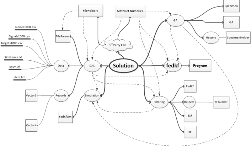
The program uses two third-party libraries: Math.Net for matrix algebra and the generation of random numbers, as well as FileHelpers to download data from CSV files. In addition, the implemented genetic algorithm engine is based on a third-party implementation of “ A Simple C # Genetic Algorithm ” (Barry Lapthorn). True, from the original implementation remains a bit.
The solution contains one project of a console application and four projects of type Class Library, containing the main logic.
GA assembly, as the name suggests, contains an implementation of genetic algorithms. It contains the structure Specimen (individual data structure) and the classes GA and SpecimenHelper. SpecimenHelper is a static class and contains static methods that simplify working with individual genes (for example, GenerateGenes, Crossover, Mutate, Print). This class also contains instances of ContinuousUniform random number generators from the Math.Net library. This generator had to be used, because I found out that the standard Random generator from .Net 4.5 assemblies generates normally distributed random numbers instead of uniformly distributed ones. For gene generation, this is quite critical.
The class GA is instance-oriented. You can create multiple instances of the optimizer with different parameters and functions of adaptation. For example, one can make the selection of the parameters of a mathematical model of sensors in one engine, and in the second one can already select the values of the covariance matrices, and through the closure “slip” into the fitness function the best at the moment assembly of the mathematical model parameters.
Simulation assembly currently contains only one static class, FedKfSim. That, in turn, contains the parameters for the simulation of a federated filter, the extension method ToFedKf for an instance of the Specimen class, which creates a federated filter for the genes of a given individual. Also this class contains a static Simulate method, in which a federated filter is created for the transferred parameters of an individual and the process of simulation of the operation of this filter is started.
Filtering assembly contains implementations of a dynamic model in the state space (class SSF), a private Kalman type filter (class KF), and a federated filter (class FedKF). The SSF class, in addition to the instance methods, contains two static methods that allow you to generate a discrete model of the state space from the coefficients of the continuous transfer function (PF). PF parameters are transmitted in MatLab notation, i.e.

The static class KFBuilder in the Filtering assembly contains auxiliary methods for generating a state space model and a private FCT using as input data the string records of the coefficients of the numerator and denominator of the continuous SF, as well as the required sampling frequency (the value inverse of the time quantization period).
The DAL assembly contains the FileParser class, used for splitting text files containing matrix data, as well as for loading signals and noise from CSV files.
For its operation, it is necessary to set the fitness function (FitnessFunction), population size (PopulationSize), number of generations (GenerationsCount), number of genes in an individual (GenomeSize), probability of crossing (CrossoverRate), probability of mutation (MutationRate).
The Initiation method is designed to generate the initial population of individuals. The method code is presented below (only the most important is left):
An important point here is the use of parallel LINQ. First, an array of indices is created from 0 to the size of the population. For this enumerable instance, a parallel query (.AsParallel ()) is created, to which a select query is already attached, in the body of which an instance of the individual will be generated and the value of its fitness will be calculated. At the end, an ordering query (.OrderBy (...)) is attached. All these were requests and this block of code will be executed quickly. The values will be updated in the following line:
what the comment says. In this case, the calculations will be performed in parallel with the use of a pool of threads; therefore, in the body of a select query, you cannot put the code to write values to any common variable (for example, to a common array). Such code will slow down the work of a parallel query (we will still face this).
On the generated individuals, an individual fitness table is calculated, which will be needed for the Roulette Wheel algorithm for sampling individuals for crossing. As can be seen from the code, each current (last) value in the table is the sum of the previous value and the current fitness. In this way, the table is filled with segments of different lengths - the greater the fitness, the greater the length of the segment (see figure below).

Due to this, using a uniformly distributed random variable ranging from zero to the sum of all adaptations, it is “honest to choose” individuals for crossing so that the most adapted individuals are chosen more often, but the “losers” also have a chance to cross. If the random number generator will produce normally distributed values (as is the case with Random in .Net 4.5), then individuals will most often be selected from the middle of the fitness table. That is why I wrote above that using ContinuousUniform from the Math.Net package was in my case a critical moment.
The next method you want to talk about is the Selection method.
In this method, selection is made. I did not choose here both parents using the roulette wheel. The first parent is selected in order from a little less than half of the most adapted individuals. The second parent is already chosen randomly. Moreover, if the second parent is close to the first in genes, the random sample is repeated until a sufficiently different parent is obtained. Then, a crossing procedure is randomly launched, which yields two individuals with mixed genes and another one, the values of which genes are selected as the average of the values of the genes of the parents.
After crossing the new individuals fitness will be double.NaN. The actualization of the values of fitness of new individuals is done again in parallel.
The last method of the GA engine that is worth telling is the RouletteSelection method.
In this method, using the half-division method, a segment is searched for in the table of adaptations, into which a randomly chosen value falls. Again, a random number is selected in the range from zero to the sum of all adaptations. The greater the fitness of a particular individual, the greater the likelihood that a randomly chosen value of fitness will fall into the segment of the table corresponding to that individual. In this way, the desired index is quite quickly.
As written earlier, the federated filter simulator is implemented by the FedKfSim class. The main method in it is the Simulate method.
In this method, an iterative process is started. At each step, a sample is taken of the pure values of the sensor signals, the noise and the reference values (the accelerations of the block without noise). Clean signals are added to noise, and this mixture is input to the Step method of a federated filter. There is also an estimate of the block accelerations from the previous step, but these values are not used in the current implementation of the private FCT. The step method of the federated filter returns an array of values — estimates of the block accelerations. The difference between them and the values of the reference will be the current estimation error. At the end of the current step, the average square of the estimation errors is calculated, and the resulting value is added to the sum of the errors. At the end of the iterations, the average error value is calculated for all process steps. The output is a number opposite to the average error.
The sequence of the application is as follows. First, the console arguments are checked. If the argument list is not empty, then an attempt is made to execute one of the valid commands.
The command “simulate” reads the gene values for which you want to generate a federated FCT from the configuration files. The “set” command is intended to change one of the values in the main configuration file of the application. The “print” command in the console displays the values of all settings from the main configuration file. The “help” command outputs basic documentation to the console.
When the application is started without arguments, the main parameters of the GA engine work are read from the configuration file, as well as the values of the matrices, signals, noises and references from the data files. After downloading all the necessary data and parameters, an instance of the optimizer is created and the evolutionary process starts.
Special attention here should be paid to the ReadSignalsAndNoises method.
It uses several separate double variables to store the values of the covariances. As I wrote above, if I used one array, then parallel tasks (Task) would be executed slowly. Actually on it I also pricked with initial implementation of this method. Within each task, I set the indices by which the resulting value of covariance should have been written in the general array. And from this point of view, the code was, it seems, safe. But it was performed extremely slowly. After replacing the array with separate variables, the calculation of the covariance matrix was significantly accelerated.
So what is done in this method? For each unique combination of two rows of noise, a separate asynchronous task is created. In these problems, the mutual variation of two random processes is calculated.
The formula is similar to the formula for calculating the variance. Only instead of the square of deviations from the mean of one random series, the product of deviations from the mean values of two separate rows is used.
Initial data
The initial data for the program are numerical rows with noises, sensor signals and the true values of the components of the block acceleration, as well as filter parameters: the matrix of cosine guides (taken from my graduation project, corresponds to the configuration of the redundant block described in one of my past articles), covariance matrix process noise (set empirically).
The reference values of the block accelerations were specified as a combination of two sinusoids. These values were recalculated into the sensor signals via the matrix of the block cosines. Sensor noise was generated in a hybrid way. I took a recording of a signal from a real sensor that was at rest while recording. Having removed the constant component from this signal, I got sensor noise in statics (this is enough for debugging algorithms). By the way, these noises turned out to be very close to white with a normal distribution. I cut these noises into short samples of 1000 values, scaled their intensities to bring the dispersions to the range [0.05..0.15]. Thus, we can say that I used real noises in my research.

The generated federated filter reduced the average noise variance by almost two times (i.e., reduced the root-mean-square error by about 1.38 times). It was possible to achieve an even more significant decrease in the variance of errors by increasing the inertia, but then the dynamic lag would increase. In my opinion, with the help of the GA, a quite efficient noise filter was generated.
I don’t have so much free time, therefore, when implementing the main functionality, there was no time for perfectionism. In some places there are security holes in the code (mainly for validating arguments), and in some places the general recommendations of the C # Code Style Guide are not followed. Surely there are blocks of code with sub-optimal performance. But despite all its flaws, it works quite well. I tested it on Intel Core i3 CPUs, and the optimization process was pretty fast. In addition, due to the use of TPL, processor resources were used quite effectively. The implemented algorithms consumed almost all the free time of the processor, but due to the normal priority of asynchronous TPL tasks, the other user programs worked without serious locks. I started the implemented program in the console and switched to working in Visual Studio 2012 with a built-in resharper, periodically switched to Outlook and MS Word, debugged the working draft in parallel in IE and Chrome browsers, without serious brakes. In general, it was a good experience using the asynchronous programming library TPL, a good result was immediately obtained without any serious difficulties.
Thanks for attention! I hope the article and the code will be useful to you.
Github sources : github.com/homoluden/fedkf-ga
UPD1 : after reading two recent articles, I also decided to join the experiment / research / adventure (call it what you want). At the end of the article added another survey - " Would you have encouraged such narrowly specialized articles on Habrahabr? With a ruble? "
Introduction
On Habré already wrote about what the Kalman Filter (FC) is, what it is for and how it is compiled (conceptually). Below are some of the available articles.
• Kalman filter
• Kalman filter - is it difficult?
• Kalman Filter - Introduction
• On the verge of augmented reality: what to prepare for developers (part 2 of 3)
• Non-orthogonal SINS for small UAVs
• Classical mechanics: on diffusers "on the fingers"
Also, there are quite a lot of articles on the use of various stochastic algorithms for optimizing nonlinear functions of many variables. Here I include evolutionary algorithms, annealing imitation, population algorithm. Links to some of the articles below.
• Simulated annealing method
• What is a genetic algorithm?
• Genetic algorithms. From theory to practice
• Genetic algorithms, image recognition
• Genetic algorithm. Just about the complicated
• Genetic algorithms for finding solutions and generating
• Genetic algorithm using the example of Robocode bot
• Genetic algorithms in MATLAB
• Population based algorithm for fish school
• Concepts of the practical use of genetic algorithms
• Review of methods for the evolution of neural networks
• TAU-Darwinism
• Natural algorithms. Bee Swarm Behavior Algorithm
• Natural algorithms. The implementation of the algorithm of the behavior of a swarm of bees
In one of my past articles ( TAU-Darwinism: Implementation in Ruby ) I presented to your attention the results of using genetic algorithms (GA) for selecting parameters of a mathematical model of a dynamic system. This article presents the results of using GA in a more complex task - the synthesis of the Kalman Filter model. Within the framework of this task, I have “set off” genetic algorithms on the parameters of the dynamics in the transition matrix (aka the Transition Matrix) FC. The GA could also be used to select the values of the covariance matrices in the FC, but I decided not to do this for now. I generated the noise myself, because the covariance matrix of measurement errors was known to me in advance. In practice, the matrix of the noise covariances of the process is never precisely known in practice; therefore, I chose its value based on the maximum sensitivity of the PC to changes in the values in the transition matrix.
Anyway, it would be easy to extend the task described here to the case of optimizing the values of the covariance matrices. It will just be necessary to implement another objective function in which the covariances matrices will be generated from the values of the individual's genes, and the value of the transition matrix will be set in advance. Thus it turns out to divide into two stages the whole process of FC synthesis:
1. Optimization of parameters of the mathematical model of FC
2. Optimization of covariance matrix values
The second stage, as I wrote above, I have not implemented yet. However, its implementation in the plans is available.
')
Formulation of the problem
So, the task. Suppose we have a certain measuring system consisting of several sensors (measuring channels). As an example, take the non-orthogonal SINS, described in another of my articles ( Non-orthogonal SINS for small UAVs ). Each of the sensors of such a system is a separate dynamic system, and at each particular time it gives one scalar measurement. There are eight measuring channels in total (according to the number of axes of sensitivity of accelerometers in a block), and there are three required parameters (components of linear acceleration of the measuring block).
What do we know about sensors? We have only recordings of signals from sensors in static mode. Those. For us, someone placed a block of accelerometers somewhere in the basement and for, say, 24 hours, recorded the values of the projection of free fall acceleration on the axis of sensitivity of the accelerometers. Also, let us be given an approximate value of the matrix of the cosine guides of the sensors in the block.
What is required of us? Create an algorithm "Filter Kalmanovsky Type" (FCT), which would give optimal estimates of the linear acceleration of the measuring unit. By optimum is meant the minimum of the variance of estimation errors and the minimum of their expectation (the minimum of the zero offset of errors).
Note: the name “Kalmanovsky Type Filter” is used, because the classic FC implies that its model coincides with the model of a real object, and the use of a different model is already called the “Lewenberger Observing Identification Device” belonging to the FCT group.
To select the parameters of the sensor models, it is proposed to use genetic algorithms. Gene values will be used as coefficients of differential equations of sensors (see “Identification Object” in Art. TAU-Darwinism ):
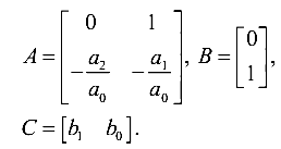
According to these coefficients, discrete models of sensors in the space-states will be built (see “Mathematical Model” in the Art. Kalman Filter — is it difficult? ):
On the basis of these models, a “private” Kalman type filter will be compiled. The assembly of several such “private” filters forms a federated FCT.
The fitness function of an individual will produce a unit divided by the average value of the squares of estimation errors:
here n is the number of steps of the filter modeling process (the number of samples in the recorded signals).
Federated Filter vs. Generalized
I have already described the concept of compiling a generalized FC (OFC) ( Kalman Filter - is it difficult? ). I will not stop in detail. The essence boils down to the fact that using the differential equations of sensors we compose models in the state space. Next, we need to make a block diagonal matrix of the OFC, joining the matrix of sensor models diagonally. Those. such matrices
should give us something like this (for the transition matrix)
where the second index of coefficients denotes the number of the sensor (measuring channel).
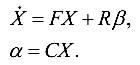
The next important point is the state vector of the FC. Roughly speaking, it contains the displacements of the pendulums of accelerometers (in the considered formulation of the problem) and the speeds of their displacements. We need to calculate what acceleration should be applied to the unit in order to bring the accelerometers into the state calculated by the FK. To do this, we must first calculate the signals of accelerometers modeled by the Kalman Filter.
Where
 | - block diagonal matrix composed of measurement matrices of sensor models |
 | - state vector of all sensors in the block |
After we have received the vector of sensor signals, it remains for us to somehow solve the overdetermined system of eight equations with three unknowns.
Where
 | - the direction cosines of the axes of sensitivity of accelerometers |
 | - the required acceleration of the measuring unit |
And then suddenly ...
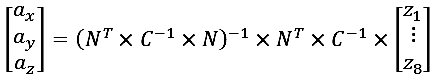
We can only compute the pseudo-inverse matrix using the Gaussian-Markov least squares method:
where N is the matrix of cosine guides (see coefficients n11, n12, ..., n83 above);
C is the covariance matrix of measurement errors (not to be confused with Sofk).
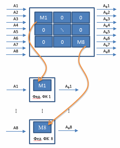
What is wrong with the OFC algorithm? In its transition matrix there are a lot of zeros for which you do not want to waste processor time. This problem is precisely solved by the Federative Algorithm of the Kalman Type Filter. The bottom line is simple. We refuse to compile a single filter that combines all the sensors at once, and implement eight separate filters for each of the sensors. Those. instead of one 16th order filter, we use 8 second order filters. Schematically it can be represented as follows.
We, like in the case of OFC, substitute the output signals of these eight “private” filters into the Gaussian-Markov OLS equation and obtain the estimates of the three components of the acceleration of the measuring unit.
What is the disadvantage of Federated Kalman type filters? They use the matrix [1x1] as the covariance matrix of measurement errors, which contains the variance of the measurement error of a single sensor. Those. instead of the covariance matrix, a scalar is used, equal to the noise dispersion of the specific sensor. Thus, the covariance of noise between the measuring channels is not taken into account. This means that such a filter should be less effective in the case of real, correlated with each other noise. This is in theory. In practice, the covariations of noise change over time, so there is no possibility to guarantee that the OFK will give a “more” optimal estimate than the federal one. It may well be that the efficiency of the OFC will not be much higher or even equal to the effectiveness of the federated filter. This, by the way, I have yet to explore.
Synthesis and Simulation Program
Solution structure
I apologize in advance for the Anglicisms - I could not find some terms from professional jargon to find the equivalent in the “great and powerful”. So, I’ll start the story about the program with an enlarged description of the structure of the solution (sorry). Then I will describe the logic of the most interesting in my opinion methods. In the end I will tell about how I generated the initial data for the program.
The structure of the solution is presented on mind-map (
The program uses two third-party libraries: Math.Net for matrix algebra and the generation of random numbers, as well as FileHelpers to download data from CSV files. In addition, the implemented genetic algorithm engine is based on a third-party implementation of “ A Simple C # Genetic Algorithm ” (Barry Lapthorn). True, from the original implementation remains a bit.
The solution contains one project of a console application and four projects of type Class Library, containing the main logic.
GA assembly, as the name suggests, contains an implementation of genetic algorithms. It contains the structure Specimen (individual data structure) and the classes GA and SpecimenHelper. SpecimenHelper is a static class and contains static methods that simplify working with individual genes (for example, GenerateGenes, Crossover, Mutate, Print). This class also contains instances of ContinuousUniform random number generators from the Math.Net library. This generator had to be used, because I found out that the standard Random generator from .Net 4.5 assemblies generates normally distributed random numbers instead of uniformly distributed ones. For gene generation, this is quite critical.
The class GA is instance-oriented. You can create multiple instances of the optimizer with different parameters and functions of adaptation. For example, one can make the selection of the parameters of a mathematical model of sensors in one engine, and in the second one can already select the values of the covariance matrices, and through the closure “slip” into the fitness function the best at the moment assembly of the mathematical model parameters.
Simulation assembly currently contains only one static class, FedKfSim. That, in turn, contains the parameters for the simulation of a federated filter, the extension method ToFedKf for an instance of the Specimen class, which creates a federated filter for the genes of a given individual. Also this class contains a static Simulate method, in which a federated filter is created for the transferred parameters of an individual and the process of simulation of the operation of this filter is started.
Filtering assembly contains implementations of a dynamic model in the state space (class SSF), a private Kalman type filter (class KF), and a federated filter (class FedKF). The SSF class, in addition to the instance methods, contains two static methods that allow you to generate a discrete model of the state space from the coefficients of the continuous transfer function (PF). PF parameters are transmitted in MatLab notation, i.e.
The static class KFBuilder in the Filtering assembly contains auxiliary methods for generating a state space model and a private FCT using as input data the string records of the coefficients of the numerator and denominator of the continuous SF, as well as the required sampling frequency (the value inverse of the time quantization period).
The DAL assembly contains the FileParser class, used for splitting text files containing matrix data, as well as for loading signals and noise from CSV files.
Genetic Algorithm Engine
For its operation, it is necessary to set the fitness function (FitnessFunction), population size (PopulationSize), number of generations (GenerationsCount), number of genes in an individual (GenomeSize), probability of crossing (CrossoverRate), probability of mutation (MutationRate).
The Initiation method is designed to generate the initial population of individuals. The method code is presented below (only the most important is left):
private void Initiation ()
private void Initiation() { //... _currGeneration = new List<Specimen>(); var newSpecies = Enumerable.Range(0, PopulationSize).AsParallel().Select(i => { var newSpec = new Specimen { Length = this.GenomeSize }; SpecimenHelper.GenerateGenes(ref newSpec); var fitness = FitnessFunction(newSpec); newSpec.Fitness = double.IsNaN(fitness) ? 0 : (double.IsInfinity(fitness) ? 1e5 : fitness); //... return newSpec; }).OrderBy(s => s.Fitness); _currGeneration = newSpecies.ToList(); // Huge load starts here :) _fitnessTable = new List<double>(); foreach (var spec in _currGeneration) { if (!_fitnessTable.Any()) { _fitnessTable.Add(spec.Fitness); } else { _fitnessTable.Add(_fitnessTable.Last() + spec.Fitness); } } TotalFitness = _currGeneration.Sum(spec => spec.Fitness); //... } An important point here is the use of parallel LINQ. First, an array of indices is created from 0 to the size of the population. For this enumerable instance, a parallel query (.AsParallel ()) is created, to which a select query is already attached, in the body of which an instance of the individual will be generated and the value of its fitness will be calculated. At the end, an ordering query (.OrderBy (...)) is attached. All these were requests and this block of code will be executed quickly. The values will be updated in the following line:
_currGeneration = newSpecies.ToList(); // Huge load starts here :)what the comment says. In this case, the calculations will be performed in parallel with the use of a pool of threads; therefore, in the body of a select query, you cannot put the code to write values to any common variable (for example, to a common array). Such code will slow down the work of a parallel query (we will still face this).
On the generated individuals, an individual fitness table is calculated, which will be needed for the Roulette Wheel algorithm for sampling individuals for crossing. As can be seen from the code, each current (last) value in the table is the sum of the previous value and the current fitness. In this way, the table is filled with segments of different lengths - the greater the fitness, the greater the length of the segment (see figure below).
Due to this, using a uniformly distributed random variable ranging from zero to the sum of all adaptations, it is “honest to choose” individuals for crossing so that the most adapted individuals are chosen more often, but the “losers” also have a chance to cross. If the random number generator will produce normally distributed values (as is the case with Random in .Net 4.5), then individuals will most often be selected from the middle of the fitness table. That is why I wrote above that using ContinuousUniform from the Math.Net package was in my case a critical moment.
The next method you want to talk about is the Selection method.
private void Selection ()
private void Selection() { var tempGenerationContainer = new ConcurrentBag<Specimen>(); //... for (int i = 0; i < this.PopulationSize / 2.5; i++) { int pidx1 = this.PopulationSize - i - 1; int pidx2 = pidx1; while (pidx1 == pidx2 || _currGeneration[pidx1].IsSimilar(_currGeneration[pidx2])) { pidx2 = RouletteSelection(); } //... var children = Rnd.NextDouble() < this.CrossoverRate ? parent1.Crossover(parent2) : new List<Specimen> { _currGeneration[pidx1], _currGeneration[pidx2] }; foreach (var ch in children.AsParallel()) { if (double.IsNaN(ch.Fitness)) { var fitness = FitnessFunction(ch); var newChild = new Specimen { Genes = ch.Genes, Length = ch.Length, Fitness = double.IsNaN(fitness) ? 0 : (double.IsInfinity(fitness) ? 1e5 : fitness) }; tempGenerationContainer.Add(newChild); } else { tempGenerationContainer.Add(ch); } } } _currGeneration = tempGenerationContainer.OrderByDescending(s => s.Fitness).Take(this.PopulationSize).Reverse().ToList(); //... } In this method, selection is made. I did not choose here both parents using the roulette wheel. The first parent is selected in order from a little less than half of the most adapted individuals. The second parent is already chosen randomly. Moreover, if the second parent is close to the first in genes, the random sample is repeated until a sufficiently different parent is obtained. Then, a crossing procedure is randomly launched, which yields two individuals with mixed genes and another one, the values of which genes are selected as the average of the values of the genes of the parents.
TODO: probably, it is necessary to replace the calculation of the average by calculating a random number in the range between the values of the parents' genes.
After crossing the new individuals fitness will be double.NaN. The actualization of the values of fitness of new individuals is done again in parallel.
foreach (var ch in children.AsParallel()) { if (double.IsNaN(ch.Fitness)) { var fitness = FitnessFunction(ch); var newChild = new Specimen { //... }; tempGenerationContainer.Add(newChild); } //... } The last method of the GA engine that is worth telling is the RouletteSelection method.
private int RouletteSelection() { double randomFitness = Rnd.NextDouble() * TotalFitness; int idx = -1; int first = 0; int last = this.PopulationSize - 1; int mid = (last - first) / 2; while (idx == -1 && first <= last) { if (randomFitness < _fitnessTable[mid]) { last = mid; } else if (randomFitness > _fitnessTable[mid]) { first = mid; } else if (randomFitness == _fitnessTable[mid]) { return mid; } mid = (first + last) / 2; // lies between i and i+1 if ((last - first) == 1) { idx = last; } } return idx; } In this method, using the half-division method, a segment is searched for in the table of adaptations, into which a randomly chosen value falls. Again, a random number is selected in the range from zero to the sum of all adaptations. The greater the fitness of a particular individual, the greater the likelihood that a randomly chosen value of fitness will fall into the segment of the table corresponding to that individual. In this way, the desired index is quite quickly.
Simulator Federated FCT
As written earlier, the federated filter simulator is implemented by the FedKfSim class. The main method in it is the Simulate method.
public static double Simulate (Specimen spec)
public static double Simulate(Specimen spec) { var fkf = spec.ToFedKf(); var meas = new double[4]; ... var err = 0.0; int lng = Math.Min(Signals.RowCount, MaxSimLength); var results = new Vector3[lng]; results[0] = new Vector3 { X = 0.0, Y = 0.0, Z = 0.0 }; for (int i = 0; i < lng; i++) { var sigRow = Signals.Row(i); var noiseRow = Noises.Row(i); var targRow = Targets.Row(i); meas[0] = sigRow[0] + noiseRow[0]; meas[1] = sigRow[1] + noiseRow[1]; meas[2] = sigRow[2] + noiseRow[2]; meas[3] = sigRow[3] + noiseRow[3]; var res = fkf.Step(meas, inps.ToColumnWiseArray()); // inps var errs = new double[] { res[0, 0] - targRow[0], res[1, 0] - targRow[1], res[2, 0] - targRow[2] }; err += (errs[0] * errs[0]) + (errs[1] * errs[1]) + (errs[2] * errs[2])/3.0; results[i] = new Vector3 { X = res[0, 0], Y = res[1, 0], Z = res[2, 0] }; ... } ... return 1/err*lng; } In this method, an iterative process is started. At each step, a sample is taken of the pure values of the sensor signals, the noise and the reference values (the accelerations of the block without noise). Clean signals are added to noise, and this mixture is input to the Step method of a federated filter. There is also an estimate of the block accelerations from the previous step, but these values are not used in the current implementation of the private FCT. The step method of the federated filter returns an array of values — estimates of the block accelerations. The difference between them and the values of the reference will be the current estimation error. At the end of the current step, the average square of the estimation errors is calculated, and the resulting value is added to the sum of the errors. At the end of the iterations, the average error value is calculated for all process steps. The output is a number opposite to the average error.
Executable application
The sequence of the application is as follows. First, the console arguments are checked. If the argument list is not empty, then an attempt is made to execute one of the valid commands.
switch (cmd) { case "simulate": case "simulation": InitializeSimulator(); FedKfSim.PrintSimResults = true; var spec = new Specimen(); SpecimenHelper.SetGenes(ref spec, ReadSimulationGenes()); FedKfSim.Simulate(spec); break; case "set": var settingName = args[1]; var settingValue = args[2]; var config = ConfigurationManager.OpenExeConfiguration(ConfigurationUserLevel.None); config.AppSettings.Settings[settingName].Value = settingValue; config.Save(ConfigurationSaveMode.Modified); ConfigurationManager.RefreshSection("appSettings"); Console.WriteLine("'{0}' set to {1}", settingName, settingValue); break; case "print": Console.WriteLine("Current settings:"); foreach (var name in ConfigurationManager.AppSettings.AllKeys.AsParallel()) { var value = ConfigurationManager.AppSettings[name]; Console.WriteLine("'{0}' => {1}", name, value); } break; case "help": case "?": case "-h": PrintHelp(); break; default: Console.Error.WriteLine(string.Format("\nARGUMENT ERROR\n'{0}' is unknown command!\n", cmd)); PrintHelp(); break; } The command “simulate” reads the gene values for which you want to generate a federated FCT from the configuration files. The “set” command is intended to change one of the values in the main configuration file of the application. The “print” command in the console displays the values of all settings from the main configuration file. The “help” command outputs basic documentation to the console.
When the application is started without arguments, the main parameters of the GA engine work are read from the configuration file, as well as the values of the matrices, signals, noises and references from the data files. After downloading all the necessary data and parameters, an instance of the optimizer is created and the evolutionary process starts.
InitializeSimulator(); var genCount = int.Parse(ConfigurationManager.AppSettings["GenerationsCount"]); var popSize = int.Parse(ConfigurationManager.AppSettings["PopulationSize"]); var crossOver = double.Parse(ConfigurationManager.AppSettings["CrossoverRate"], FileParser.NumberFormat); var mutRate = double.Parse(ConfigurationManager.AppSettings["MutationRate"], FileParser.NumberFormat); var maxGeneVal = double.Parse(ConfigurationManager.AppSettings["MaxGeneValue"], FileParser.NumberFormat); var minGeneVal = double.Parse(ConfigurationManager.AppSettings["MinGeneValue"], FileParser.NumberFormat); var genomeLength = int.Parse(ConfigurationManager.AppSettings["GenomeLength"]); SpecimenHelper.SimilarityThreshold = double.Parse( ConfigurationManager.AppSettings["SimilarityThreshold"], FileParser.NumberFormat); var ga = new Ga(genomeLength) { FitnessFunction = FedKfSim.Simulate, Elitism = true, GenerationsCount = genCount, PopulationSize = popSize, CrossoverRate = crossOver, MutationRate = mutRate }; FedKfSim.PrintSimResults = false; ga.Go(maxGeneVal, minGeneVal); Special attention here should be paid to the ReadSignalsAndNoises method.
private static void ReadSignalsAndNoises ()
private static void ReadSignalsAndNoises() { var noisesPath = ConfigurationManager.AppSettings["NoisesFilePath"]; var signalsPath = ConfigurationManager.AppSettings["SignalsFilePath"]; var targetsPath = ConfigurationManager.AppSettings["TargetsFilePath"]; FedKfSim.Noises = new DenseMatrix(FileParser.Read4ColonFile(noisesPath)); FedKfSim.Signals = new DenseMatrix(FileParser.Read4ColonFile(signalsPath)); FedKfSim.Targets = new DenseMatrix(FileParser.Read3ColonFile(targetsPath)); var measCov = new DenseMatrix(4); double c00 = 0, c01 = 0, c02 = 0, c03 = 0, c11 = 0, c12 = 0, c13 = 0, c22 = 0, c23 = 0, c33 = 0; Vector<double> v1 = new DenseVector(1); Vector<double> v2 = new DenseVector(1); Vector<double> v3 = new DenseVector(1); Vector<double> v4 = new DenseVector(1); var s1 = new DescriptiveStatistics(new double[1]); var s2 = new DescriptiveStatistics(new double[1]); var s3 = new DescriptiveStatistics(new double[1]); var s4 = new DescriptiveStatistics(new double[1]); var t00 = Task.Run(() => { v1 = FedKfSim.Noises.Column(0); s1 = new DescriptiveStatistics(v1); c00 = s1.Variance; }); var t11 = Task.Run(() => { v2 = FedKfSim.Noises.Column(1); s2 = new DescriptiveStatistics(v2); c11 = s2.Variance; }); var t22 = Task.Run(() => { v3 = FedKfSim.Noises.Column(2); s3 = new DescriptiveStatistics(v3); c22 = s3.Variance; }); var t33 = Task.Run(() => { v4 = FedKfSim.Noises.Column(3); s4 = new DescriptiveStatistics(v4); c33 = s4.Variance; }); Task.WaitAll(new[] { t00, t11, t22, t33 }); var t01 = Task.Run(() => c01 = CalcVariance(v1, s1.Mean, v2, s2.Mean, FedKfSim.Noises.RowCount)); var t02 = Task.Run(() => c02 = CalcVariance(v1, s1.Mean, v3, s3.Mean, FedKfSim.Noises.RowCount)); var t03 = Task.Run(() => c03 = CalcVariance(v1, s1.Mean, v4, s4.Mean, FedKfSim.Noises.RowCount)); var t12 = Task.Run(() => c12 = CalcVariance(v2, s2.Mean, v3, s3.Mean, FedKfSim.Noises.RowCount)); var t13 = Task.Run(() => c13 = CalcVariance(v2, s2.Mean, v4, s4.Mean, FedKfSim.Noises.RowCount)); var t23 = Task.Run(() => c23 = CalcVariance(v3, s3.Mean, v4, s4.Mean, FedKfSim.Noises.RowCount)); Task.WaitAll(new[] { t01, t02, t03, t12, t13, t23 }); measCov[0, 0] = c00; measCov[0, 1] = c01; measCov[0, 2] = c02; measCov[0, 3] = c03; measCov[1, 0] = c01; measCov[1, 1] = c11; measCov[1, 2] = c12; measCov[1, 3] = c13; measCov[2, 0] = c02; measCov[2, 1] = c12; measCov[2, 2] = c22; measCov[2, 3] = c23; measCov[3, 0] = c03; measCov[3, 1] = c13; measCov[3, 2] = c23; measCov[3, 3] = c33; FedKfSim.SensorsOutputCovariances = measCov; } It uses several separate double variables to store the values of the covariances. As I wrote above, if I used one array, then parallel tasks (Task) would be executed slowly. Actually on it I also pricked with initial implementation of this method. Within each task, I set the indices by which the resulting value of covariance should have been written in the general array. And from this point of view, the code was, it seems, safe. But it was performed extremely slowly. After replacing the array with separate variables, the calculation of the covariance matrix was significantly accelerated.
So what is done in this method? For each unique combination of two rows of noise, a separate asynchronous task is created. In these problems, the mutual variation of two random processes is calculated.
private static double CalcVariance(IEnumerable<double> v1, double mean1, IEnumerable<double> v2, double mean2, int length) { var zipped = v1.Take(length).Zip(v2.Take(length), (i1, i2) => new[] { i1, i2 }); var sum = zipped.AsParallel().Sum(z => (z[0] - mean1) * (z[1] - mean2)); return sum / (length - 1); } The formula is similar to the formula for calculating the variance. Only instead of the square of deviations from the mean of one random series, the product of deviations from the mean values of two separate rows is used.
Initial data
The initial data for the program are numerical rows with noises, sensor signals and the true values of the components of the block acceleration, as well as filter parameters: the matrix of cosine guides (taken from my graduation project, corresponds to the configuration of the redundant block described in one of my past articles), covariance matrix process noise (set empirically).
The reference values of the block accelerations were specified as a combination of two sinusoids. These values were recalculated into the sensor signals via the matrix of the block cosines. Sensor noise was generated in a hybrid way. I took a recording of a signal from a real sensor that was at rest while recording. Having removed the constant component from this signal, I got sensor noise in statics (this is enough for debugging algorithms). By the way, these noises turned out to be very close to white with a normal distribution. I cut these noises into short samples of 1000 values, scaled their intensities to bring the dispersions to the range [0.05..0.15]. Thus, we can say that I used real noises in my research.
results
The generated federated filter reduced the average noise variance by almost two times (i.e., reduced the root-mean-square error by about 1.38 times). It was possible to achieve an even more significant decrease in the variance of errors by increasing the inertia, but then the dynamic lag would increase. In my opinion, with the help of the GA, a quite efficient noise filter was generated.
Conclusion
I don’t have so much free time, therefore, when implementing the main functionality, there was no time for perfectionism. In some places there are security holes in the code (mainly for validating arguments), and in some places the general recommendations of the C # Code Style Guide are not followed. Surely there are blocks of code with sub-optimal performance. But despite all its flaws, it works quite well. I tested it on Intel Core i3 CPUs, and the optimization process was pretty fast. In addition, due to the use of TPL, processor resources were used quite effectively. The implemented algorithms consumed almost all the free time of the processor, but due to the normal priority of asynchronous TPL tasks, the other user programs worked without serious locks. I started the implemented program in the console and switched to working in Visual Studio 2012 with a built-in resharper, periodically switched to Outlook and MS Word, debugged the working draft in parallel in IE and Chrome browsers, without serious brakes. In general, it was a good experience using the asynchronous programming library TPL, a good result was immediately obtained without any serious difficulties.
Thanks for attention! I hope the article and the code will be useful to you.
Github sources : github.com/homoluden/fedkf-ga
Source: https://habr.com/ru/post/178453/
All Articles