Briefly about hydrodynamics: stability theory
Well, we continue. Let's move on closer to what hydrodynamics looks quite enticing, and try to add as many beautiful and relatively beautiful images as possible.
The text will be written a little more theory on the example of the problem of the stability of the flow in a flat channel. There are a lot of such tasks in reality - in layers and in limited cavities of different shapes, in vertical, horizontal and inclined layers, in ordinary fluid and porous medium, in conducting fluid under the influence of a magnetic field and in solution of some salt under the action of temperature, cavities under the influence of an arbitrarily directed vibration, at the interface of two liquids ... In general, just listing all the sublevels of hydrodynamics can take a couple of hours, and it is unlikely that we can remember everything. And also several examples of purely hydrodynamic instability of currents will be shown, without the influence of additional factors (images about 700 kB).
The previous posts were written to provide the mathematical and semantic basis of formulas in further posts.
')
Briefly about hydrodynamics: do you remember how it all began?
Briefly about hydrodynamics: equations of motion
Briefly about hydrodynamics: energy conservation
The theory of stability in general is a very wide area, which can be found both in theoretical mechanics and in theories of linear and non-linear oscillations (where it is most developed). The theory of hydrodynamic stability, due to the specificity of the object being studied and the corresponding systems of equations, is kept by it in a special way. Consider a couple of the simplest (and perhaps the most fundamental) examples.
Let us have some arbitrary incompressible viscous flow. It is quite natural that it is described by the Navier-Stokes equations:

The equations are still in dimensional form. But it is convenient to dimension them for further work, since This operation reduces the number of parameters and allows you to immediately determine which mechanisms are most significant in the behavior of the system. The dimensioning procedure is reduced to rescaling all variables in such a way as to minimize the number of parameters. Most often, the determining factor is the time scale - we can choose the characteristic time as its unit, during which the flow with its characteristic speed will pass some characteristic length of the channel (for brevity, we call it kinematic, since it is determined by the school relationship time = distance / speed, but this term is nowhere to be found), pulse transfer time (viscous time), heat (thermal time), external influence, etc. For the equations of motion in the channel, it is most convenient to take the kinematic times, indicate some conditional scale of speed, length, and choose the scale for pressure, based on the greatest simplification of the equation:

When substituting the scales in the equation and reducing to the density and factor before the nonlinear term, we see that all coefficients become equal to unity, except for the viscous term. There arises a combination of parameters expressing the inverse Reynolds number:

The second equation of its kind does not change when it is dimensionless. Thus, the Reynolds number is the only parameter that determines the behavior of the system.

Chic is that only this one parameter is responsible for the laminarity or turbulence of the flow, while the equations do not change a bit.
Suppose further that we have some stationary, constant in time flow with speed , and there are some infinitesimal perturbations of this flow:

You can safely substitute the speed and pressure in this form into the system, discard everything that contains only stationary fields of speed and pressure, since they satisfy the equations by themselves, and neglecting the nonlinear term is the most important move in the whole theory. Since we assume the perturbations are infinitesimal, then the term of the form becomes infinitesimal second order. Therefore, saying that we work in an area where the perturbations can still be considered small (that is, at the very beginning of the development of future instabilities), we can safely discard the nonlinearity. As a result, two linear equations remain, albeit with variable coefficients:

This system is the basic system of equations of the linear theory of hydrodynamic stability, and describes the most common situations. Let us now look at one more specific situation - the stability of a plane-parallel flow in a channel. Everything happens in the ( x , z ) plane, and the channel along the y axis is infinitely long — that is, a purely two-dimensional flow. Let the stationary solution have only one component, depending on the transverse coordinate of the channel, and the disturbances - two components:

We also take (since the equations are linear and the typical solution for them is the exponent) the exponential dependence on time . Such perturbations are usually called “normal”, although the history of this term is rather vague. Substituting the indicated dependence and writing down the equations in projections on the axes, we obtain a system for plane perturbations. At the same time, the coefficients in it do not depend on the x coordinate, therefore we can additionally assume that the perturbations are periodic along this axis - in fact, it is close to the decomposition in the Fourier series and the consideration of only one component:
  . It turns out that such a system is already from ordinary differential equations (the prime denotes the derivative with respect to z ):

Lowering the intermediate transformations, simple but taking up a couple of pages, let us point out that this system can be reduced to one equation for the velocity component w :
If in it to write the complex increment and enter the phase velocity of perturbations
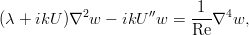
get the equation, known as the Orr-Sommerfeld equation:

The entire linear theory of the hydrodynamic stability of flows is based on this equation. True, there are no exact solutions for it, regardless of the type of stationary flow and boundary conditions, although outwardly everything looks extremely simple and the problem is closed.
In solving this problem there were different approaches. For example, Rayleigh in the approximation of large Reynolds numbers simply neglected the right side. Of course, this is not always correct, since the fourth derivatives can easily compensate for the denominator. True, the equation still could not be solved, but it turned out to prove the theorem on the necessary condition for the stability of the flow . True, for the Poiseuille flow this condition is not fulfilled, but it can still be unstable.
It is possible, in the same approximation, to extend the decomposition in the inverse Reynolds number as a small parameter. In the zero order of this decomposition, the mentioned Rayleigh problem turns out, and if you go a little further, you can catch two curves on the parameter plane ( k , Re), between which the region of flow instability will be enclosed, in which the disturbances increase and lead to the destruction of the stationary profile . At first, for the Poiseuille flow, Heisenberg tried to solve this problem (the same Werner Heisenberg, the creator of matrix quantum mechanics), but he failed to completely decompose. As a result, in 1944, the Chinese patient Lin Jia-Jiao took up the case, stretched the decompositions a little further and extrapolated both curves, which were closed into one. It turned out about the following (solid line):

In fact, this chart is already a bit different for another system - instead of the usual liquid, the authors considered suspension of some fibers in the channel, but its meaning is the same and there are no significant qualitative differences from Lin's theory (illustration from You Zhenjianga, Lin Jianzhonga, Yu Zhaoshengb Fluid Dynamics Research, Volume 34 (4), 2004, pp. 251–271. In general, the Poiseuille flow, for almost any liquid, has such stability properties that only emphasizes the fundamental nature of Lin's results.
Below are the pictures, mostly drawn from the “Album of liquid and gas flows” (M. Van Dyke) and simply from the network, with a few comments on specific problem statements.
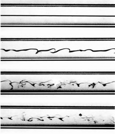
This experiment was carried out by Reynolds in 1883. The photos were taken on the same installation, which was safely preserved about a hundred years later. From top to bottom in the photos, the flow rate increases. A thin colored stream is introduced into the stream, which allows perfect visualization of the flow.
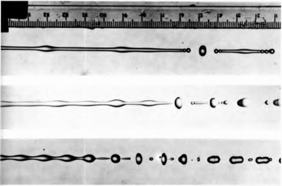
Very elegant instability that we can observe every day. It is enough to open the faucet so that the trickle is even and thin, but long enough. Due to the interaction of random perturbations and capillary forces, the continuous stream tends to break into small drops, since it is energetically more profitable. Here the liquid is disturbed by the loudspeaker to which the output tube is connected. The wavelength of the disturbance in the lower picture is close to the theoretical critical value.


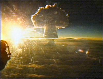
A rather uncomplicated situation - on the surface of a light liquid, we pour a heavy one. It is quite obvious that the heavy one will strive to “fall” down, although for the time being, surface tension can withstand the process. But when the movement begins, it happens very beautifully, both in laboratories and calculations, and in nature (the second picture is reversed, as conceived by its author and photo artist).
A similar phenomenon is observed if there are two areas in the medium with very different pressures — the substance “pushes” through the interface between them and gives rise to structures similar to simple “falling through”.
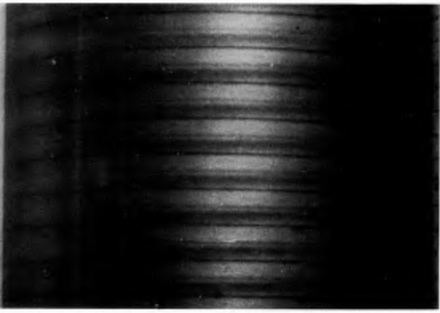

Another version of the instability, something of the origin of such Rayleigh-Taylor. The fluid is located between two coaxial cylinders and is driven into rapid rotation. Due to centripetal accelerations, annular cells with opposite flow directions are formed in the medium initially fixed relative to the cylinder walls.
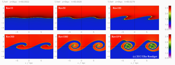
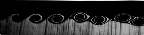

And one more version of instability. Also, physically, very simple. We have two streams of immiscible liquids moving opposite to each other. Or just with different speeds - i.e. at the interface between them, there is a jump in speed, due to which the perturbations of the surface are deformed, twisted and produce intricate vortexes, and then completely mix the fluids. It also looks interesting in calculations, in an experimental setup, and in nature.
Here, of course, not the whole spectrum of possible instabilities is shown — the region is inexhaustible, and contains a huge spectrum of still-unexplored phenomena and their features. The next post will be about convection and the corresponding instabilities caused by temperature heterogeneity in the system.
The text will be written a little more theory on the example of the problem of the stability of the flow in a flat channel. There are a lot of such tasks in reality - in layers and in limited cavities of different shapes, in vertical, horizontal and inclined layers, in ordinary fluid and porous medium, in conducting fluid under the influence of a magnetic field and in solution of some salt under the action of temperature, cavities under the influence of an arbitrarily directed vibration, at the interface of two liquids ... In general, just listing all the sublevels of hydrodynamics can take a couple of hours, and it is unlikely that we can remember everything. And also several examples of purely hydrodynamic instability of currents will be shown, without the influence of additional factors (images about 700 kB).
The previous posts were written to provide the mathematical and semantic basis of formulas in further posts.
')
Briefly about hydrodynamics: do you remember how it all began?
Briefly about hydrodynamics: equations of motion
Briefly about hydrodynamics: energy conservation
The theory of stability in general is a very wide area, which can be found both in theoretical mechanics and in theories of linear and non-linear oscillations (where it is most developed). The theory of hydrodynamic stability, due to the specificity of the object being studied and the corresponding systems of equations, is kept by it in a special way. Consider a couple of the simplest (and perhaps the most fundamental) examples.
Stability of two-dimensional flow
Let us have some arbitrary incompressible viscous flow. It is quite natural that it is described by the Navier-Stokes equations:
The equations are still in dimensional form. But it is convenient to dimension them for further work, since This operation reduces the number of parameters and allows you to immediately determine which mechanisms are most significant in the behavior of the system. The dimensioning procedure is reduced to rescaling all variables in such a way as to minimize the number of parameters. Most often, the determining factor is the time scale - we can choose the characteristic time as its unit, during which the flow with its characteristic speed will pass some characteristic length of the channel (for brevity, we call it kinematic, since it is determined by the school relationship time = distance / speed, but this term is nowhere to be found), pulse transfer time (viscous time), heat (thermal time), external influence, etc. For the equations of motion in the channel, it is most convenient to take the kinematic times, indicate some conditional scale of speed, length, and choose the scale for pressure, based on the greatest simplification of the equation:
When substituting the scales in the equation and reducing to the density and factor before the nonlinear term, we see that all coefficients become equal to unity, except for the viscous term. There arises a combination of parameters expressing the inverse Reynolds number:
The second equation of its kind does not change when it is dimensionless. Thus, the Reynolds number is the only parameter that determines the behavior of the system.
Chic is that only this one parameter is responsible for the laminarity or turbulence of the flow, while the equations do not change a bit.
Suppose further that we have some stationary, constant in time flow with speed
, and there are some infinitesimal perturbations of this flow:You can safely substitute the speed and pressure in this form into the system, discard everything that contains only stationary fields of speed and pressure, since they satisfy the equations by themselves, and neglecting the nonlinear term is the most important move in the whole theory. Since we assume the perturbations are infinitesimal, then the term of the form
becomes infinitesimal second order. Therefore, saying that we work in an area where the perturbations can still be considered small (that is, at the very beginning of the development of future instabilities), we can safely discard the nonlinearity. As a result, two linear equations remain, albeit with variable coefficients:This system is the basic system of equations of the linear theory of hydrodynamic stability, and describes the most common situations. Let us now look at one more specific situation - the stability of a plane-parallel flow in a channel. Everything happens in the ( x , z ) plane, and the channel along the y axis is infinitely long — that is, a purely two-dimensional flow. Let the stationary solution have only one component, depending on the transverse coordinate of the channel, and the disturbances - two components:
We also take (since the equations are linear and the typical solution for them is the exponent) the exponential dependence on time
. Such perturbations are usually called “normal”, although the history of this term is rather vague. Substituting the indicated dependence and writing down the equations in projections on the axes, we obtain a system for plane perturbations. At the same time, the coefficients in it do not depend on the x coordinate, therefore we can additionally assume that the perturbations are periodic along this axis - in fact, it is close to the decomposition in the Fourier series and the consideration of only one component: . It turns out that such a system is already from ordinary differential equations (the prime denotes the derivative with respect to z ):Lowering the intermediate transformations, simple but taking up a couple of pages, let us point out that this system can be reduced to one equation for the velocity component w :
If in it to write the complex increment and enter the phase velocity of perturbations
get the equation, known as the Orr-Sommerfeld equation:
The entire linear theory of the hydrodynamic stability of flows is based on this equation. True, there are no exact solutions for it, regardless of the type of stationary flow and boundary conditions, although outwardly everything looks extremely simple and the problem is closed.
In solving this problem there were different approaches. For example, Rayleigh in the approximation of large Reynolds numbers simply neglected the right side. Of course, this is not always correct, since the fourth derivatives can easily compensate for the denominator. True, the equation still could not be solved, but it turned out to prove the theorem on the necessary condition for the stability of the flow . True, for the Poiseuille flow this condition is not fulfilled, but it can still be unstable.
It is possible, in the same approximation, to extend the decomposition in the inverse Reynolds number as a small parameter. In the zero order of this decomposition, the mentioned Rayleigh problem turns out, and if you go a little further, you can catch two curves on the parameter plane ( k , Re), between which the region of flow instability will be enclosed, in which the disturbances increase and lead to the destruction of the stationary profile
. At first, for the Poiseuille flow, Heisenberg tried to solve this problem (the same Werner Heisenberg, the creator of matrix quantum mechanics), but he failed to completely decompose. As a result, in 1944, the Chinese patient Lin Jia-Jiao took up the case, stretched the decompositions a little further and extrapolated both curves, which were closed into one. It turned out about the following (solid line):In fact, this chart is already a bit different for another system - instead of the usual liquid, the authors considered suspension of some fibers in the channel, but its meaning is the same and there are no significant qualitative differences from Lin's theory (illustration from You Zhenjianga, Lin Jianzhonga, Yu Zhaoshengb Fluid Dynamics Research, Volume 34 (4), 2004, pp. 251–271. In general, the Poiseuille flow, for almost any liquid, has such stability properties that only emphasizes the fundamental nature of Lin's results.
Examples of instabilities
Below are the pictures, mostly drawn from the “Album of liquid and gas flows” (M. Van Dyke) and simply from the network, with a few comments on specific problem statements.
Development of the Poiseuil flow instability
This experiment was carried out by Reynolds in 1883. The photos were taken on the same installation, which was safely preserved about a hundred years later. From top to bottom in the photos, the flow rate increases. A thin colored stream is introduced into the stream, which allows perfect visualization of the flow.
Liquid column instability (Rayleigh-Plato problem)
Very elegant instability that we can observe every day. It is enough to open the faucet so that the trickle is even and thin, but long enough. Due to the interaction of random perturbations and capillary forces, the continuous stream tends to break into small drops, since it is energetically more profitable. Here the liquid is disturbed by the loudspeaker to which the output tube is connected. The wavelength of the disturbance in the lower picture is close to the theoretical critical value.
Rayleigh-Taylor Instability
A rather uncomplicated situation - on the surface of a light liquid, we pour a heavy one. It is quite obvious that the heavy one will strive to “fall” down, although for the time being, surface tension can withstand the process. But when the movement begins, it happens very beautifully, both in laboratories and calculations, and in nature (the second picture is reversed, as conceived by its author and photo artist).
A similar phenomenon is observed if there are two areas in the medium with very different pressures — the substance “pushes” through the interface between them and gives rise to structures similar to simple “falling through”.
Whirlwinds of taylor
Another version of the instability, something of the origin of such Rayleigh-Taylor. The fluid is located between two coaxial cylinders and is driven into rapid rotation. Due to centripetal accelerations, annular cells with opposite flow directions are formed in the medium initially fixed relative to the cylinder walls.
Kelvin-Helmholtz instability
And one more version of instability. Also, physically, very simple. We have two streams of immiscible liquids moving opposite to each other. Or just with different speeds - i.e. at the interface between them, there is a jump in speed, due to which the perturbations of the surface are deformed, twisted and produce intricate vortexes, and then completely mix the fluids. It also looks interesting in calculations, in an experimental setup, and in nature.
Here, of course, not the whole spectrum of possible instabilities is shown — the region is inexhaustible, and contains a huge spectrum of still-unexplored phenomena and their features. The next post will be about convection and the corresponding instabilities caused by temperature heterogeneity in the system.
Source: https://habr.com/ru/post/178145/
All Articles