Mathematical model of the engine Lego NXT
Good afternoon, dear colleagues. In this article I want to share with you my methodical practices that I use in the course “Theory of Automatic Control” at the Department of MSE at NRU ITMO.
The main task that I set for myself was to unite theoretical knowledge to solve a practical problem. This task was the management of drives Lego robot. There is an extra reason to play with toys, and it is easier for students to perceive the stern matan ... Here is an example of the description of this set: habrahabr.ru/post/166449 .
Let's go in order, for a start it was necessary to make an adequate mathematical model of the engine. And already here I ran into a problem: the manufacturers did not indicate the technical characteristics of the engines in the set. A search on Google gives a number of options (for example, nxt-unroller.blogspot.ru/2011/01/motor-controller-with-feed-forward-for.html or philohome.com/nxtmotor/nxtmotor.htm ), but I need It was to get the characteristics of the engines that were used in the robot. Here the knowledge of physics and theoretical mechanics came in handy.
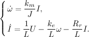
We make the Lagrange-Euler equation and take into account the effect of back-EMF in the rotor winding of a direct current motor (DC motor), we get:
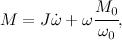
where w is the angular velocity of rotation of the motor, w0 is the idling speed, M is the torque developed by the engine, M0 is the starting torque, J is the inertia moment of the rotor of the motor. The solution of the differential equation is the following expression:
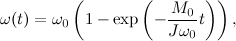
where J * w0 / M0 = Tm, Tm is the electromechanical constant of the engine.
The function of changing the angle over time will be the integral of the speed function with regard to the initial conditions:
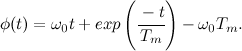
Just the same we need it.
Further, it was necessary to write a program that would remove the characteristic of overclocking of the DC motor described by the indicated equation. For this, I used nxcEditor for Linux and Bricxcc for Windows. At the output, I received a file containing the angle values and the corresponding time readings.
The data from the engine was processed in Scilab (open analog of Matlab), obtaining the values of the electromechanical constant and steady-state engine speed using the least squares method, which will be equal to aa (2) = Tm = 0.081 [s] and aa (1) = w0 = 14.7 [rad / sec] respectively.
And check the validity of the obtained values by applying to the engine control in the form of a sinusoid (the image shows the graphs of the reaction of the mathematical model and the real engine, the graph of the real engine floats down due to the resistance in the motor circuit, when rotating clockwise and against, which affects power key):

Now it was easy to proceed to the calculation of the Kostructive engine constants, which are necessary to control its torque. For this, I used the system of motor equations describing electrical processes:
where ke, km are constructive constants, U = 7 [V] is the control voltage, L = 0.0047 [Hn] is the winding inductance, Rr = 6 [Ohm] is the resistance of the robot winding ,. Measured the starting current I = 0.9 [A] (measured when the rotor is locked) and calculated the moment of inertia of the rotor. Using the following formula, I got the starting torque given by the engine:

In equation i = 48 is the reduction coefficient. The current transfer ratio was equal to 0.42, dividing the starting torque at the output shaft to the starting current

The coefficient of transfer of back-electromotive force equal to 0.48, calculated as the ratio of the steady-state angular velocity to the supplied voltage

The next step is to program the control of the angle of rotation of the DPT. Used for this proportional regulator. Software implementation is as follows:
And now comes the moment of truth, as far as our calculated model corresponds to the real situation (the model was going to Scilab Xcos).
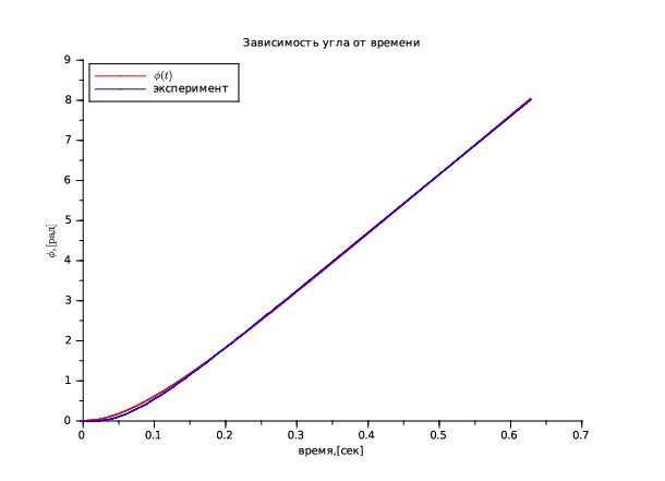
I give a model and experimental curve:
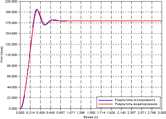
As you can see, everything converges with a deviation of no more than 3%.
Such simple experiments performed with our own hands make it possible to understand the basics of mathematical modeling and control theory.
In turn, ready to share a manual for the performance of work.
I am pleased to hear your comments and suggestions.
The main task that I set for myself was to unite theoretical knowledge to solve a practical problem. This task was the management of drives Lego robot. There is an extra reason to play with toys, and it is easier for students to perceive the stern matan ... Here is an example of the description of this set: habrahabr.ru/post/166449 .
Let's go in order, for a start it was necessary to make an adequate mathematical model of the engine. And already here I ran into a problem: the manufacturers did not indicate the technical characteristics of the engines in the set. A search on Google gives a number of options (for example, nxt-unroller.blogspot.ru/2011/01/motor-controller-with-feed-forward-for.html or philohome.com/nxtmotor/nxtmotor.htm ), but I need It was to get the characteristics of the engines that were used in the robot. Here the knowledge of physics and theoretical mechanics came in handy.
We make the Lagrange-Euler equation and take into account the effect of back-EMF in the rotor winding of a direct current motor (DC motor), we get:
where w is the angular velocity of rotation of the motor, w0 is the idling speed, M is the torque developed by the engine, M0 is the starting torque, J is the inertia moment of the rotor of the motor. The solution of the differential equation is the following expression:
where J * w0 / M0 = Tm, Tm is the electromechanical constant of the engine.
The function of changing the angle over time will be the integral of the speed function with regard to the initial conditions:
Just the same we need it.
Further, it was necessary to write a program that would remove the characteristic of overclocking of the DC motor described by the indicated equation. For this, I used nxcEditor for Linux and Bricxcc for Windows. At the output, I received a file containing the angle values and the corresponding time readings.
The data from the engine was processed in Scilab (open analog of Matlab), obtaining the values of the electromechanical constant and steady-state engine speed using the least squares method, which will be equal to aa (2) = Tm = 0.081 [s] and aa (1) = w0 = 14.7 [rad / sec] respectively.
data=read("/home/kasper/Number.txt",-1,2); time=(data(:,2)-data(1,2))/1000; angle=data(:,1)*%pi/180; angle=angle'; time=time'; f=[time;angle]; function e=G(a, z), e = z(2) - a(1)*(z(1)-a(2)+a(2)*%e^(-z(1)/a(2))); endfunction a0=[1;4]; [aa,er]=datafit(G,f,a0); model=aa(1)*(time+aa(2)*(%e^(-time/aa(2))-1)); xtitle(' ','time','$\dot\phi,[\frac{}{}]$'); plot2d(time,model,[5]); a=gca(); a.children.children(1).thickness=2; plot2d(time,angle,[2]); a.children.children(1).thickness=2; a.children.children(1).text=["$\dot\phi(t)$"]; And check the validity of the obtained values by applying to the engine control in the form of a sinusoid (the image shows the graphs of the reaction of the mathematical model and the real engine, the graph of the real engine floats down due to the resistance in the motor circuit, when rotating clockwise and against, which affects power key):
Now it was easy to proceed to the calculation of the Kostructive engine constants, which are necessary to control its torque. For this, I used the system of motor equations describing electrical processes:
where ke, km are constructive constants, U = 7 [V] is the control voltage, L = 0.0047 [Hn] is the winding inductance, Rr = 6 [Ohm] is the resistance of the robot winding ,. Measured the starting current I = 0.9 [A] (measured when the rotor is locked) and calculated the moment of inertia of the rotor. Using the following formula, I got the starting torque given by the engine:
In equation i = 48 is the reduction coefficient. The current transfer ratio was equal to 0.42, dividing the starting torque at the output shaft to the starting current
The coefficient of transfer of back-electromotive force equal to 0.48, calculated as the ratio of the steady-state angular velocity to the supplied voltage
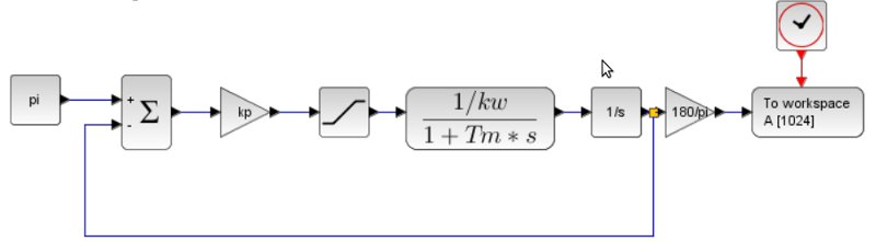
The next step is to program the control of the angle of rotation of the DPT. Used for this proportional regulator. Software implementation is as follows:
#define NEED_ANGLE 180 #define WORK_TIME 3000 #define KOL_EXPS 3 #define PORT OUT_A #define KP 14 task main() { int angle_now, battery_voltage, power_percent, time = 0; int i, str_size, file_size = 8224; byte file; string str = "3lab.txt"; float need_voltage, angle_diff; DeleteFile(str); CreateFile(str, file_size, file); while(time < WORK_TIME) { angle_now = MotorRotationCount(PORT); time = CurrentTick() - FirstTick(); angle_diff = NEED_ANGLE - angle_now; angle_diff = angle_diff * 3.1415 / 180; need_voltage = KP * angle_diff; need_voltage *= 1000; battery_voltage = BatteryLevel(); power_percent = need_voltage / battery_voltage * 100; if(abs(power_percent) > 100) power_percent = 100 * sign(power_percent); OnFwd(PORT, power_percent); str = NumToStr(angle_now) + " " + NumToStr(time); WriteLnString(file, str, str_size); Wait(MS_5); } Off(PORT); CloseFile(file); } And now comes the moment of truth, as far as our calculated model corresponds to the real situation (the model was going to Scilab Xcos).
I give a model and experimental curve:
As you can see, everything converges with a deviation of no more than 3%.
Such simple experiments performed with our own hands make it possible to understand the basics of mathematical modeling and control theory.
In turn, ready to share a manual for the performance of work.
I am pleased to hear your comments and suggestions.
')
Source: https://habr.com/ru/post/178103/
All Articles