Probabilistic models: examples and pictures
Today is the second series of the cycle begun last time ; then we talked about directed graphical probabilistic models, drew the main pictures of this science and discussed what dependencies and independence they correspond to. Today - a series of illustrations to the material of the past; We will discuss several important and interesting models, draw pictures corresponding to them and see how they correspond to the factorizations of the joint distribution of all variables.

To begin with, I briefly repeat the previous text: we have already talked about the naive Bayes classifier in this blog. In naive Bayes, an additional assumption is made about the conditional independence of attributes (words) subject to the condition:

The result is a complex posterior distribution. managed to rewrite as

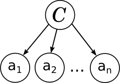
And what a picture of this model corresponds to:
')
Everything is exactly as we said last time: individual words in a document are associated with a variable of a category by a diverging link; this shows that they are conditionally independent under the condition of this category. Learning naive bayes is to train the parameters of individual factors: a priori distribution on categories p ( C ) and conditional distributions of individual parameters .
.
One more note about the pictures before moving on. Very often in models there are a large number of variables of the same type that are associated with other variables by the same distributions (possibly with different parameters). To make the picture easier to read and understand, so that it doesn’t have innumerable dots and things like “well, here is a complete bipartite graph with dots, well, you understand,” it is convenient to combine the same type variables into so-called “plates”. To do this, draw a rectangle into which one typical representative of the variable being propagated is placed; somewhere in the corner of the rectangle it is convenient to sign how many copies are meant:

And the general model of all documents (without dies, we did not draw it) will consist of several copies of this graph and, accordingly, look like this:
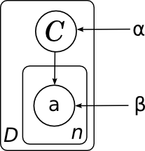
Here I explicitly drew the distribution parameters on the categories α and the parameters are the probabilities of words in each category β. Since these parameters do not have a separate factor in the decomposition, the network node does not correspond to them, but it is often convenient to also depict them for clarity. In this case, the picture means that different copies of the variable C were generated from the same distribution p ( C ), and different copies of the words were generated from the same distribution, parametrized by the category value (i.e., β is the matrix probabilities of different words in different categories).
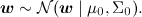
We will continue with another model that you may vaguely recall from a course of mathematical statistics - linear regression. The essence of the model is simple: we assume that the variable y , which we want to predict, is obtained from the feature vector x as some linear function with weights w (bold font will denote vectors - this is generally accepted, and in html it will be more convenient for me than every time to draw an arrow) and normally distributed noise:

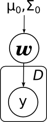
The model assumes that some data set is available to us, dataset D. It consists of separate implementations of this regression itself, and (important!) It is assumed that these implementations were generated independently. In addition, a priori distribution of parameters is often introduced in linear regression — for example, the normal distribution
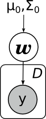
Then we come to this picture:

Here I explicitly drew the parameters of the prior distribution μ 0 and Σ 0 . Pay attention - linear regression is very similar in structure to naive bayes.
With dies, the same thing will look even simpler:
What are the main tasks that are solved in linear regression? The first task is to find the posterior distribution on w , i.e. learn how to recalculate the distribution of w with the available data ( x , y ) of D ; mathematically we have to calculate the distribution parameters

In graphic models, the variables are usually hatched, the values of which are known; Thus, the task is to recalculate the distribution w for such a column with evidence:
The second main task (something even more basic) is to calculate the predictive distribution, estimate the new value of y at some new point. Mathematically, this task looks significantly more complicated than the previous one - now it is necessary to integrate by the posterior distribution

And graphically, not so much changes - we draw a new variable that we want to predict, but the task is still the same: with some evidence (from dataset) recalculate the distribution of some other variable in the model, only now it is not w , but y * :

Another widely known and popular class of probabilistic models is hidden Markov models (HMM). They are used in speech recognition, for fuzzy search for substrings and in other similar applications. The hidden Markov model is a Markov chain (a sequence of random variables, where each value x t + 1 depends only on the previous x t and under the condition x t conditionally independent with the previous x tk ), in which we cannot observe hidden states, but only see some observables y t that depend on the current state. For example, in speech recognition, hidden states are phonemes that you want to say (this is a simplification, in fact, each phoneme is an entire model, but it will come down for illustration), and the observed ones are sound waves that reach the discriminator. The picture is this:

This picture is enough to solve the problem of applying the already hidden Markov model: according to the existing model (consisting of transition probabilities between hidden states A , initial distribution of chain π and distribution parameters of observable B ) and given sequence of observables, find the most likely sequence of hidden states; i.e., for example, in a ready-made speech recognition system, recognize a new sound file. And if you need to train the model parameters, it is better to clearly draw them in the picture, so that it is clear that the same parameters are involved in all transitions:

Another model that we already talked about - LDA (latent Dirichlet allocation, latent Dirichlet placement). This is a model for thematic modeling, in which each document is represented not by a single topic, as in naive Bayes, but by a discrete distribution on possible topics. In the same text, we have already described the LDA generative model - how to generate a document in the finished LDA model:
Now we understand what the corresponding picture will look like (it was also in that blog post, and again I will copy it from Wikipedia , but the essence of the picture here is exactly the same as ours above):

In a series of posts ( 1 , 2 , 3 , 4 ) we talked about one of the main tools of collaborative filtering - the singular decomposition of matrices, SVD.
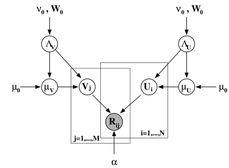
We looked for the SVD-decomposition by the gradient descent method: we constructed the error function, counted the gradient from it, went down it. However, it is possible to formulate a general probabilistic problem formulation, which is usually called PMF (probabilistic matrix factorization). To do this, we need to introduce a priori distributions for the vectors of features of users and products:
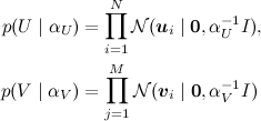
(where I is the identity matrix), and then, as in a regular SVD, present ratings as noisy linear combinations of user and product attributes:
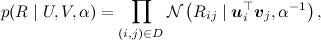
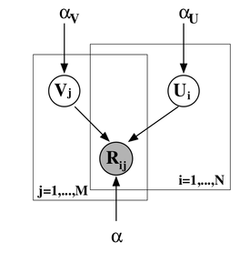
where the product is taken from the ratings present in the training set. It turns out such a picture (the picture is taken from the article [Salakhutdinov, Mnih, 2009] ):
You can add another level of Bayesian inference and train at the same time hyper-parameters of the distribution of signs for users and products; I will not go into it now, but I will simply provide the corresponding picture (from the same article ) - perhaps, it is still possible to talk about this in more detail.
Another example that is personally close to me is that once Alexander Syrotkin and I improved one of the Bayesian rating systems; Perhaps later in the blog we will talk about rating systems in more detail. But here I’ll just give the simplest example - how does the Elo rating for chess players work? If you do not go into approximations and magic constants, the essence is very simple: what is a rating in general? We would like the rating to be the measure of the strength of the game; however, it is quite obvious that the strength of the game from one game to another may change quite strongly under the influence of external and internal random factors. Thus, in fact, the strength of a game of a participant in a particular game (comparison of these forces determines the outcome of the game) is a random variable, the “true power” of a game of a chess player is its expectation, and rating is our inaccurate assessment of this expectation. . For the time being, we will consider the simplest case in which the player’s playing power in a particular game is normally distributed around his true power with some constant fixed dispersion in advance (Elo’s rating does just that - hence his magic constant “a chess player with a strength of 200 points gains more an average of 0.75 points per game ”). Before each game, we have some a priori estimates of the strength of the game of each chess player; Suppose that the prior distribution is also normal, with the parameters μ 1 , σ 1 and μ 2 , σ 2, respectively. Our task - knowing the result of the party, recalculate these parameters. The picture is this:
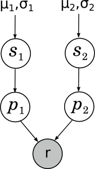
Here s i (skill) is the “true power of the game” of a chess player, p i (performance) is his strength of the game shown in this particular game, and r is a rather interesting random variable showing the result of the game, which is obtained from comparing p 1 and p 2 . More about this today will not.
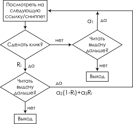
And I will end with another close example to me - models of the behavior of Internet users in search engines. Again, I won’t go into detail - maybe we’ll come back to this, but for now you can read, for example, our review article with Alexander Fishkov - just consider one such model for example. We are trying to simulate what the user does when receiving search results. Viewing links and clicks are treated as random events; For a specific request session, the variable E i denotes viewing the description of the link to the document shown at position i , C i - click on this position. We introduce a simplifying assumption: suppose that the process of viewing descriptions always starts from the first position and is strictly linear. Position is viewed only if all previous positions have been viewed. As a result, our virtual user reads the links from top to bottom, if he liked (which depends on the relevance of the link), clicks, and if the document really turns out to be relevant, the user leaves and no longer returns; curious, but true: a good event for a search engine is when a user leaves and does not return as quickly as possible, and if he returns to the list, he could not find what he was looking for.
The result is the so-called cascading click model (cascading click model, CCM); in it, the user follows this flowchart:
And in the form of a Bayesian network, you can draw it like this:
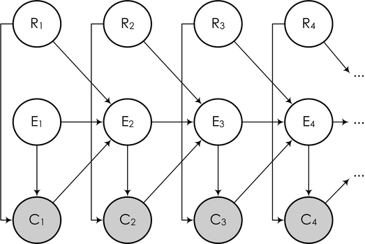
Here the subsequent events of E i (this event is “user read the next snippet”, from the word examine) depend on whether there was a click on the previous link, and if so, whether the link was really relevant. The task is again described as above: we observe part of the variables (user clicks), and must, based on clicks, train the model and draw conclusions about the relevance of each link (in order to further reorder the links according to their true relevance), i.e. . about the values of some other variables in the model.
In this article, we looked at a few examples of probabilistic models, the logic of which is easy to “read” from their directed graphical models. In addition, we were convinced that what we usually want from a probabilistic model can be represented as one fairly well-defined problem — in a directed graphical model, recalculate the distribution of some variables with known values of some other variables. However, logic is logic, but how, in fact, to teach? How to solve this problem? About this - in the following series.
Naive Bayes Classifier
To begin with, I briefly repeat the previous text: we have already talked about the naive Bayes classifier in this blog. In naive Bayes, an additional assumption is made about the conditional independence of attributes (words) subject to the condition:
The result is a complex posterior distribution.
managed to rewrite asAnd what a picture of this model corresponds to:
')
Everything is exactly as we said last time: individual words in a document are associated with a variable of a category by a diverging link; this shows that they are conditionally independent under the condition of this category. Learning naive bayes is to train the parameters of individual factors: a priori distribution on categories p ( C ) and conditional distributions of individual parameters
.One more note about the pictures before moving on. Very often in models there are a large number of variables of the same type that are associated with other variables by the same distributions (possibly with different parameters). To make the picture easier to read and understand, so that it doesn’t have innumerable dots and things like “well, here is a complete bipartite graph with dots, well, you understand,” it is convenient to combine the same type variables into so-called “plates”. To do this, draw a rectangle into which one typical representative of the variable being propagated is placed; somewhere in the corner of the rectangle it is convenient to sign how many copies are meant:
And the general model of all documents (without dies, we did not draw it) will consist of several copies of this graph and, accordingly, look like this:
Here I explicitly drew the distribution parameters on the categories α and the parameters are the probabilities of words in each category β. Since these parameters do not have a separate factor in the decomposition, the network node does not correspond to them, but it is often convenient to also depict them for clarity. In this case, the picture means that different copies of the variable C were generated from the same distribution p ( C ), and different copies of the words were generated from the same distribution, parametrized by the category value (i.e., β is the matrix probabilities of different words in different categories).
Linear regression
We will continue with another model that you may vaguely recall from a course of mathematical statistics - linear regression. The essence of the model is simple: we assume that the variable y , which we want to predict, is obtained from the feature vector x as some linear function with weights w (bold font will denote vectors - this is generally accepted, and in html it will be more convenient for me than every time to draw an arrow) and normally distributed noise:
The model assumes that some data set is available to us, dataset D. It consists of separate implementations of this regression itself, and (important!) It is assumed that these implementations were generated independently. In addition, a priori distribution of parameters is often introduced in linear regression — for example, the normal distribution
Then we come to this picture:
Here I explicitly drew the parameters of the prior distribution μ 0 and Σ 0 . Pay attention - linear regression is very similar in structure to naive bayes.
With dies, the same thing will look even simpler:
What are the main tasks that are solved in linear regression? The first task is to find the posterior distribution on w , i.e. learn how to recalculate the distribution of w with the available data ( x , y ) of D ; mathematically we have to calculate the distribution parameters
In graphic models, the variables are usually hatched, the values of which are known; Thus, the task is to recalculate the distribution w for such a column with evidence:
The second main task (something even more basic) is to calculate the predictive distribution, estimate the new value of y at some new point. Mathematically, this task looks significantly more complicated than the previous one - now it is necessary to integrate by the posterior distribution
And graphically, not so much changes - we draw a new variable that we want to predict, but the task is still the same: with some evidence (from dataset) recalculate the distribution of some other variable in the model, only now it is not w , but y * :
Hidden Markov Models
Another widely known and popular class of probabilistic models is hidden Markov models (HMM). They are used in speech recognition, for fuzzy search for substrings and in other similar applications. The hidden Markov model is a Markov chain (a sequence of random variables, where each value x t + 1 depends only on the previous x t and under the condition x t conditionally independent with the previous x tk ), in which we cannot observe hidden states, but only see some observables y t that depend on the current state. For example, in speech recognition, hidden states are phonemes that you want to say (this is a simplification, in fact, each phoneme is an entire model, but it will come down for illustration), and the observed ones are sound waves that reach the discriminator. The picture is this:
This picture is enough to solve the problem of applying the already hidden Markov model: according to the existing model (consisting of transition probabilities between hidden states A , initial distribution of chain π and distribution parameters of observable B ) and given sequence of observables, find the most likely sequence of hidden states; i.e., for example, in a ready-made speech recognition system, recognize a new sound file. And if you need to train the model parameters, it is better to clearly draw them in the picture, so that it is clear that the same parameters are involved in all transitions:
Lda
Another model that we already talked about - LDA (latent Dirichlet allocation, latent Dirichlet placement). This is a model for thematic modeling, in which each document is represented not by a single topic, as in naive Bayes, but by a discrete distribution on possible topics. In the same text, we have already described the LDA generative model - how to generate a document in the finished LDA model:
- choose the length of the document N (this is not drawn on the graph - it is not that part of the model);
- choose vector
 - the vector of "severity" of each topic in this document;
 - for each of the N words w :
- choose a topic
 by distribution
  ;
; - choose a word
 with probabilities given in β.
- choose a topic
Now we understand what the corresponding picture will look like (it was also in that blog post, and again I will copy it from Wikipedia , but the essence of the picture here is exactly the same as ours above):
SVD and PMF
In a series of posts ( 1 , 2 , 3 , 4 ) we talked about one of the main tools of collaborative filtering - the singular decomposition of matrices, SVD.
We looked for the SVD-decomposition by the gradient descent method: we constructed the error function, counted the gradient from it, went down it. However, it is possible to formulate a general probabilistic problem formulation, which is usually called PMF (probabilistic matrix factorization). To do this, we need to introduce a priori distributions for the vectors of features of users and products:
(where I is the identity matrix), and then, as in a regular SVD, present ratings as noisy linear combinations of user and product attributes:
where the product is taken from the ratings present in the training set. It turns out such a picture (the picture is taken from the article [Salakhutdinov, Mnih, 2009] ):
You can add another level of Bayesian inference and train at the same time hyper-parameters of the distribution of signs for users and products; I will not go into it now, but I will simply provide the corresponding picture (from the same article ) - perhaps, it is still possible to talk about this in more detail.
Bayesian rating systems
Another example that is personally close to me is that once Alexander Syrotkin and I improved one of the Bayesian rating systems; Perhaps later in the blog we will talk about rating systems in more detail. But here I’ll just give the simplest example - how does the Elo rating for chess players work? If you do not go into approximations and magic constants, the essence is very simple: what is a rating in general? We would like the rating to be the measure of the strength of the game; however, it is quite obvious that the strength of the game from one game to another may change quite strongly under the influence of external and internal random factors. Thus, in fact, the strength of a game of a participant in a particular game (comparison of these forces determines the outcome of the game) is a random variable, the “true power” of a game of a chess player is its expectation, and rating is our inaccurate assessment of this expectation. . For the time being, we will consider the simplest case in which the player’s playing power in a particular game is normally distributed around his true power with some constant fixed dispersion in advance (Elo’s rating does just that - hence his magic constant “a chess player with a strength of 200 points gains more an average of 0.75 points per game ”). Before each game, we have some a priori estimates of the strength of the game of each chess player; Suppose that the prior distribution is also normal, with the parameters μ 1 , σ 1 and μ 2 , σ 2, respectively. Our task - knowing the result of the party, recalculate these parameters. The picture is this:
Here s i (skill) is the “true power of the game” of a chess player, p i (performance) is his strength of the game shown in this particular game, and r is a rather interesting random variable showing the result of the game, which is obtained from comparing p 1 and p 2 . More about this today will not.
Internet user behavior
And I will end with another close example to me - models of the behavior of Internet users in search engines. Again, I won’t go into detail - maybe we’ll come back to this, but for now you can read, for example, our review article with Alexander Fishkov - just consider one such model for example. We are trying to simulate what the user does when receiving search results. Viewing links and clicks are treated as random events; For a specific request session, the variable E i denotes viewing the description of the link to the document shown at position i , C i - click on this position. We introduce a simplifying assumption: suppose that the process of viewing descriptions always starts from the first position and is strictly linear. Position is viewed only if all previous positions have been viewed. As a result, our virtual user reads the links from top to bottom, if he liked (which depends on the relevance of the link), clicks, and if the document really turns out to be relevant, the user leaves and no longer returns; curious, but true: a good event for a search engine is when a user leaves and does not return as quickly as possible, and if he returns to the list, he could not find what he was looking for.
The result is the so-called cascading click model (cascading click model, CCM); in it, the user follows this flowchart:
And in the form of a Bayesian network, you can draw it like this:
Here the subsequent events of E i (this event is “user read the next snippet”, from the word examine) depend on whether there was a click on the previous link, and if so, whether the link was really relevant. The task is again described as above: we observe part of the variables (user clicks), and must, based on clicks, train the model and draw conclusions about the relevance of each link (in order to further reorder the links according to their true relevance), i.e. . about the values of some other variables in the model.
Conclusion and conclusions
In this article, we looked at a few examples of probabilistic models, the logic of which is easy to “read” from their directed graphical models. In addition, we were convinced that what we usually want from a probabilistic model can be represented as one fairly well-defined problem — in a directed graphical model, recalculate the distribution of some variables with known values of some other variables. However, logic is logic, but how, in fact, to teach? How to solve this problem? About this - in the following series.
Source: https://habr.com/ru/post/177889/
All Articles