Experimenting Experimental Data
The other day there was a problem to program the device for measuring the flow rate of air. As a measuring element - the sensor is not clear what manufacturer, there are no characteristics or any adequate parameters. There was no choice, I had to remove the calibration characteristics and output the transfer function “ADC-flow counts”.
Since the sensor, like almost any measuring instrument, is very sensitive to temperature, I needed to remove a family of characteristics (minimum 3) for different temperatures.
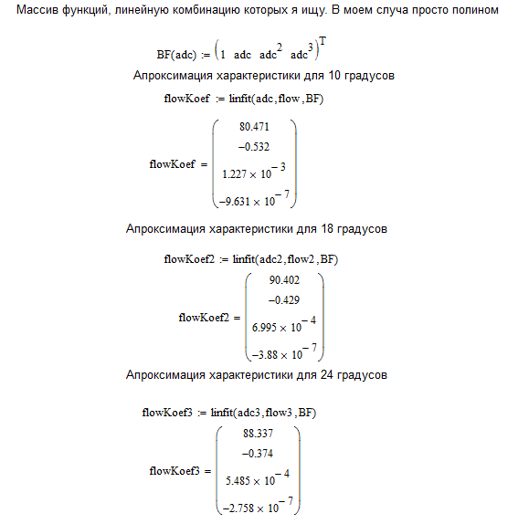
Data can be entered into MathCad in different ways, I preferred to do this in the form of transposed row vectors:

After this, it is necessary to define the type of the approximating function by an “volitional” solution and approximate each calibration characteristic. So, my characteristics are successfully approximated by a third-degree polynomial using the linfit function, which looks for a solution in the form of linear combinations of arbitrary functions, I obtained coefficients for three polynomials:
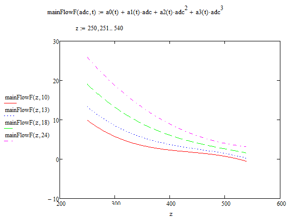
To see how “successfully” the experimental data are modeled by the resulting polynomial, we can construct a graph:

Now, in order to introduce a temperature correction, it is necessary to find the dependence of each of the polynomial coefficients on temperature, i.e. do all of the above for the coefficients only. In the role of experimental data will now be the coefficients and temperature values. I really wanted that the temperature dependence was linear, it is possible to use the linfit function unnecessarily for linear approximation, but still:

Finally, the desired dependency appears as follows:
Commenting on the result, I note that it turned out not very well, frankly disgusting. Characteristics were initially poorly removed, the lack of a normal stand affected. In general, the calibration task is far from amateurish; you cannot do it on your lap. But I wanted to tell you about the approach.
Since the sensor, like almost any measuring instrument, is very sensitive to temperature, I needed to remove a family of characteristics (minimum 3) for different temperatures.
Data can be entered into MathCad in different ways, I preferred to do this in the form of transposed row vectors:
After this, it is necessary to define the type of the approximating function by an “volitional” solution and approximate each calibration characteristic. So, my characteristics are successfully approximated by a third-degree polynomial using the linfit function, which looks for a solution in the form of linear combinations of arbitrary functions, I obtained coefficients for three polynomials:
To see how “successfully” the experimental data are modeled by the resulting polynomial, we can construct a graph:
Now, in order to introduce a temperature correction, it is necessary to find the dependence of each of the polynomial coefficients on temperature, i.e. do all of the above for the coefficients only. In the role of experimental data will now be the coefficients and temperature values. I really wanted that the temperature dependence was linear, it is possible to use the linfit function unnecessarily for linear approximation, but still:
Finally, the desired dependency appears as follows:
Commenting on the result, I note that it turned out not very well, frankly disgusting. Characteristics were initially poorly removed, the lack of a normal stand affected. In general, the calibration task is far from amateurish; you cannot do it on your lap. But I wanted to tell you about the approach.
')
Source: https://habr.com/ru/post/177461/
All Articles