Multiple variable polynomials and Haskell’s Buchberger algorithm
In this article I want to talk about how to implement the algorithms associated with the Gröbner bases, in Haskell. I hope someone my ideas and explanations will be useful. I'm not going to go into theory, so the reader should be familiar with the concepts of the polynomial ring, the ideal ring and the ideal basis. I advise you to read this book of ICNMO, in it all the necessary theory is described in detail.
The main subject of the paper is the Gröbner bases of ideals of polynomial rings of several variables. This concept arises in the study of systems of polynomial equations. At the end of the article I will show by example how to apply these ideas.
The most important result that this theory gives is a good way to solve polynomial systems of equations of several variables. Even if you are not familiar with higher algebra or Haskell, I advise you to read this article, since these very methods of solution are explained at the level accessible to the student, and the whole theory is needed only for substantiation. You can safely skip everything related to higher algebra, and just learn how to solve systems of equations.
')
If you are interested, please under the cat.
I apologize for the pictures - this is rendered by latex, and how to make habr understand
Sets, on the elements of which two operations can be defined - “addition” and “multiplication”, which correspond to a certain set of rules (axioms), are called rings in algebra. Polynomials in several variables whose coefficients are real numbers form a ring, denoted by , regarding ordinary school operations of addition and multiplication of polynomials. The ideal of a ring is its subset, the difference of two elements of which lies in it and the product of any of its elements and an arbitrary element of the ring lies in this subset. The simplest example of an ideal is a set of multiples of five numbers as an ideal in the ring of integers. See for yourself that this is ideal. If it worked out, there would be no further problems.
Further we will consider only ideals in the ring of polynomials. Some finite set of polynomials is called an ideal basis if any polynomial from an ideal is represented as
  where
where  - some polynomials. This fact is recorded as:
  . Hilbert's theorem on a basis gives a remarkable result — every ideal (in a ring of polynomials) has a finite basis. This allows you to work in any situation just to work with finite bases of ideals.
Now we will consider systems of equations of the following form:
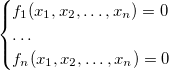
Let's call the ideal of this system the ideal. . It is known from algebra that any polynomial lying in the ideal  , vanishes on any solution of the source system. And further, if
  - another ideal basis then the system
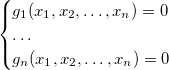
has the same set of solutions as the original one. From all this it follows that if we succeed in finding a basis in the ideal of a system that is simpler than the original, then the problem of solving the system itself is simplified.
In a magical way, such a basis exists - it is called the Gröbner basis of the ideal. By definition, this is such a basis that the division procedure with the remainder (about it later) for any polynomial of the ideal will yield a zero remainder. If we construct it, then one of its polynomials, at least in most cases, will depend on only one variable, which will allow us to solve the entire system by successive substitution.
The last thing we need is -mold and criterion -Buchberger pair. Choose some "good" way of arranging monomials (for details - in the book) and denote by
  the leading term (with respect to this ordering) of a polynomial
  and through
  - least common multiple of monomials
  and
and  . Then polynomial from and
  called the following structure:

Proved (criterion -pair), that the ideal basis is its Gröbner basis if and only if - a polynomial from any pair of its members gives the remainder 0 when dividing by a basis (how this is done will be explained later). This immediately prompts the algorithm for constructing such a basis:
This is the Buchberger algorithm - the main subject of this article. On this with mathematics everything, you can go. If you do not understand something, you should look at Wikipedia or a book, although the further narrative does not require knowledge of higher algebra.
Let's start building a representation of polynomials with monomials. A monomial is characterized by only two things - a coefficient and a set of degrees of variables. We assume that there are variables ,
,  and so on. Then monomial
  has a coefficient of 1 and degree
  - coefficient 2 and degree
We describe the type of “monomial” as an algebraic data type consisting of a coefficient (type “
We will need to compare monomials with each other, so it's time to write an embodiment of the
The
I will write functions that are similar to
Now we are ready to describe the actual type of polynomials. For this, a
This time, the
We agree on the future that the monomials in this list will always be stored in descending order (in the sense of our definition of the
The simplest operations are LT, checks for equality to zero and multiplication by a number. From our agreement on the ordering of monomials, it follows that the highest monom is always at the top of the list and can be obtained with the help of
Two monomials will be called similar if they differ only in coefficients. For them, the sum is determined - you just need to add the coefficients, and the degrees remain unchanged.
To multiply two monomials, simply add the powers of each of the variables. This operation is very easy to accomplish with the great
The addition of polynomials is much more interesting. We will solve this problem recursively. Trivial cases - the sum of two zero polynomials (empty lists) is equal to the zero polynomial. The sum of any polynomial and zero is equal to it. Now we can consider both polynomials to be non-zero, which means that each of them can be divided into the senior member and the others - the “tail”. There are two cases:
It remains to be noted that as a result of this recursive procedure, an ordered polynomial will again be obtained, and write the actual code.
Multiplication of polynomials is obtained in an absolutely natural way. It is very easy to multiply a monomial by a polynomial - just multiply it by each of the monomials using
That's all, we have implemented the basic actions on polynomials, which means we can move on!
Let's say that monomial divided into monomial if there is such a monomial  , what
  . Obviously, this is true only if each variable is included in no less than . Therefore, the check for divisibility can be implemented using the familiar
Note that now the type of the coefficient should allow division - the
The division algorithm of a polynomial on a basis with the remainder is essentially a simple school column division. Among the polynomials of the basis, the first such polynomial is chosen, that the eldest member of the dividend is divided into its senior member, then this polynomial multiplied by the quotient of its older members is subtracted from the dividend. The result of the subtraction is taken as a new dividend and the process is repeated. If the senior member is not divided into any of the senior members of the base, the division is completed and the last divisible element is called the remainder.
Our main division procedure, let's call it
Since we do not have a function for subtraction, we simply multiply the second polynomial by -1 and add them - everything is simple! And here is the whole division algorithm:
The
Here we come to the main part of this article - the implementation of the Buchberger algorithm. The only thing we don’t have yet is the functions to get polynomial Its implementation is very simple, as is the auxiliary function for finding the smallest common multiple of monomials:
Here both polynomials are simply multiplied by the corresponding monomials, with the second additionally also having a minus one, as in the case of division with the remainder.
I am sure that there are many ways to implement this algorithm. I also do not pretend that my implementation is sufficiently optimal or simple. But I like it and it works, and that's all it takes.
The approach I used can be called dynamic. We divide our basis into two parts - the one in which we have already checked (and added) -polynomials from all pairs - “
As soon as the second part is empty, the first will contain the Gröbner basis. The advantage of this solution is that they will not be considered -polynomials from those pairs from which they are already counted and verified. The key function in this process is
Surely this can be replaced by sly
The polynomial -polynomials of each polynomial of the second part only from the first, due to the displacements of polynomials between parts. It remains to be noted that to obtain the Gröbner basis from this one, it is enough to place one of its polynomials in the first part, the rest in the second and apply the
All these theoretical constructions seem completely useless without demonstrating the practical application of these methods. As an example, consider the problem of finding the intersection point of three circles - the simplest case of positioning on the map. We write the equations of circles as a system of equations:
 .
.
After opening the brackets, we get the following:

Construct the Gröbner basis (I used the
In a miraculous way, we got two linear equations that quickly give the answer - the point (7.5). You can check that it lies on all three circles. So, we have reduced the solution of a system of three complex square equations to two simple linear ones. Gröbner bases are really useful tools for such tasks.
In fact, this result can still be improved. -polynomials need to be counted only for those pairs of polynomials whose higher members are not mutually simple - that is, their least common multiple is not just their product. In some sources about this case they say "polynomials have a link ". Add this optimization to our
If a polynomial got into the final basis, the senior member of which is divided into the senior member of some other polynomial from the basis, then it can be excluded. The basis obtained after eliminating all such polynomials is called the Gröbner minimal basis. You can also consider a polynomial, an arbitrary member of which is divided into the senior member of some other polynomial. In this case, we replace this polynomial by the remainder of division by another. The basis in which all possible operations of this type are carried out is called reduced . As an exercise, implement minimization and reduction of the base.
In conclusion, I want to say thank you to everyone who read this article to the end. I know that my narration was somewhat chaotic, and the code is not ideal (and, perhaps, incomprehensible), but I still hope that I have interested someone with Gröbner bases. I would be very pleased if someone can find the use of my work in any real tasks.
All code from the article is available as gist .
The main subject of the paper is the Gröbner bases of ideals of polynomial rings of several variables. This concept arises in the study of systems of polynomial equations. At the end of the article I will show by example how to apply these ideas.
The most important result that this theory gives is a good way to solve polynomial systems of equations of several variables. Even if you are not familiar with higher algebra or Haskell, I advise you to read this article, since these very methods of solution are explained at the level accessible to the student, and the whole theory is needed only for substantiation. You can safely skip everything related to higher algebra, and just learn how to solve systems of equations.
')
If you are interested, please under the cat.
I apologize for the pictures - this is rendered by latex, and how to make habr understand
style="width:...;height=...;" I do not know. If you tell the better way, be sure to redo it.1 The most necessary concepts from algebra
Sets, on the elements of which two operations can be defined - “addition” and “multiplication”, which correspond to a certain set of rules (axioms), are called rings in algebra. Polynomials in several variables whose coefficients are real numbers form a ring, denoted by
, regarding ordinary school operations of addition and multiplication of polynomials. The ideal of a ring is its subset, the difference of two elements of which lies in it and the product of any of its elements and an arbitrary element of the ring lies in this subset. The simplest example of an ideal is a set of multiples of five numbers as an ideal in the ring of integers. See for yourself that this is ideal. If it worked out, there would be no further problems.Further we will consider only ideals in the ring of polynomials. Some finite set of polynomials
is called an ideal basis if any polynomial from an ideal is represented as where - some polynomials. This fact is recorded as: . Hilbert's theorem on a basis gives a remarkable result — every ideal (in a ring of polynomials) has a finite basis. This allows you to work in any situation just to work with finite bases of ideals.Now we will consider systems of equations of the following form:
Let's call the ideal of this system the ideal.
. It is known from algebra that any polynomial lying in the ideal , vanishes on any solution of the source system. And further, if - another ideal basis then the systemhas the same set of solutions as the original one. From all this it follows that if we succeed in finding a basis in the ideal of a system that is simpler than the original, then the problem of solving the system itself is simplified.
In a magical way, such a basis exists - it is called the Gröbner basis of the ideal. By definition, this is such a basis that the division procedure with the remainder (about it later) for any polynomial of the ideal will yield a zero remainder. If we construct it, then one of its polynomials, at least in most cases, will depend on only one variable, which will allow us to solve the entire system by successive substitution.
The last thing we need is
-mold and criterion -Buchberger pair. Choose some "good" way of arranging monomials (for details - in the book) and denote by the leading term (with respect to this ordering) of a polynomial and through - least common multiple of monomials and . Then polynomial from and called the following structure:Proved (criterion
-pair), that the ideal basis is its Gröbner basis if and only if - a polynomial from any pair of its members gives the remainder 0 when dividing by a basis (how this is done will be explained later). This immediately prompts the algorithm for constructing such a basis:- For each pair of base polynomials compose them -policy and share it with the remainder on the basis.
- If all residues are zero, the Gröbner basis is obtained. Otherwise, add all nonzero residues to the base and return to step 1.
This is the Buchberger algorithm - the main subject of this article. On this with mathematics everything, you can go. If you do not understand something, you should look at Wikipedia or a book, although the further narrative does not require knowledge of higher algebra.
2 Representation of polynomials in several Haskell variables
Let's start building a representation of polynomials with monomials. A monomial is characterized by only two things - a coefficient and a set of degrees of variables. We assume that there are variables
, and so on. Then monomial has a coefficient of 1 and degree [2,3,1] , while the monomial - coefficient 2 and degree [0,0,3] . Pay attention to zero degrees! They are critical for implementing all the other methods. In general, we require that the lists of powers of all monomials (within the same task) have the same length. This will greatly simplify our work.We describe the type of “monomial” as an algebraic data type consisting of a coefficient (type “
c ”) and a list of degrees (each type “ a ”): data Monom ca = M c [a] deriving (Eq) We will need to compare monomials with each other, so it's time to write an embodiment of the
Ord class. I will use the usual lexicographical ordering in powers, since it is very simple and at the same time corresponds to the rules of "good" ordering of monomials. We will also write the embodiment of the Show class just for the convenience of working with our system. instance (Eq c, Ord a) => Ord (Monom ca) where compare (M _ asl) (M _ asr) = compare asl asr instance (Show a, Show c, Num a, Num c, Eq a, Eq c) => Show (Monom ca) where show (M c as) = (if c == 1 then "" else show c) ++ (intercalate "*" $ map showOne $ (filter (\(p,_) -> p /= 0) $ zip as [1..])) where showOne (p,i) = "x" ++ (show i) ++ (if p == 1 then "" else "^" ++ (show p)) The
show function tries to be “smart”: it does not show the coefficient, if it is equal to 1, and it does not show variables of zero degree, nor does it show the first degree of variables. Like this: *Main> M 2 [0,1] 2x2 *Main> M 1 [2,2] x1^2*x2^2 I will write functions that are similar to
show , all the time, so it’s worth explaining exactly how it works - I’m sure it scared anyone. Using zip as [1..] glue each power with its own variable number, then with filter (
(p _) -> p /= 0) filter (
(p _) -> p /= 0) filter (
(p _) -> p /= 0) get rid of zero degrees, we turn the description of each variable into a string through showOne and, finally, we glue everything together, interspersed with multiplication icons, using intercalate from Data.ListNow we are ready to describe the actual type of polynomials. For this, a
newtype wrapper over a regular list will do: newtype Polynom ca = P [Monom ca] deriving (Eq) instance (Show a, Show c, Num a, Num c, Eq a, Eq c) => Show (Polynom ca) where show (P ms) = intercalate " + " $ map show ms This time, the
show function is simple, since all the dirty work is already hidden in the type of monomials. It works like this: *Main> P [M 1 [3,1], M 1 [2,2], M 1 [1,1]] x1^3*x2 + x1^2*x2^2 + x1*x2 We agree on the future that the monomials in this list will always be stored in descending order (in the sense of our definition of the
Ord incarnation). This will make it possible to realize some things much easier.3 Polynomial operations
The simplest operations are LT, checks for equality to zero and multiplication by a number. From our agreement on the ordering of monomials, it follows that the highest monom is always at the top of the list and can be obtained with the help of
head . A monomial is considered to be zero if its coefficient is zero, and a polynomial is considered to contain no monomials. Well, multiplication by a constant simply changes the coefficient: lt :: Polynom ca -> Monom ca lt (P as) = head as zero :: (Num c, Eq c) => Monom ca -> Bool zero (M c _) = c == 0 zeroP :: Polynom ca -> Bool zeroP (P as) = null as scale :: (Num c) => c -> Monom ca -> Monom ca scale c' (M c as) = M (c*c') as Two monomials will be called similar if they differ only in coefficients. For them, the sum is determined - you just need to add the coefficients, and the degrees remain unchanged.
similar :: (Eq a) => Monom ca -> Monom ca -> Bool similar (M _ asl) (M _ asr) = asl == asr addSimilar :: (Num c) => Monom ca -> Monom ca -> Monom ca addSimilar (M cl as) (M cr _) = M (cl+cr) as To multiply two monomials, simply add the powers of each of the variables. This operation is very easy to accomplish with the great
zipWith . I think the code speaks for itself: mulMono :: (Num a, Num c) => Monom ca -> Monom ca -> Monom ca mulMono (M cl asl) (M cr asr) = M (cl*cr) (zipWith (+) asl asr) The addition of polynomials is much more interesting. We will solve this problem recursively. Trivial cases - the sum of two zero polynomials (empty lists) is equal to the zero polynomial. The sum of any polynomial and zero is equal to it. Now we can consider both polynomials to be non-zero, which means that each of them can be divided into the senior member and the others - the “tail”. There are two cases:
- Older members are similar. In this case, add them and add the result (if it is non-zero) to the sum of the tails.
- Older members are not alike. Then pick the bigger one. Our ordering condition guarantees that there is no similar monomial in the tails of both polynomials. Consequently, we can fold the tail of the chosen polynomial with another, and then add to its beginning this largest monomial.
It remains to be noted that as a result of this recursive procedure, an ordered polynomial will again be obtained, and write the actual code.
addPoly :: (Eq a, Eq c, Num c, Ord a) => Polynom ca -> Polynom ca -> Polynom ca addPoly (P l) (P r) = P $ go lr where go [] [] = [] go as [] = as go [] bs = bs go (a:as) (b:bs) = if similar ab then if (zero $ addSimilar ab) then go as bs else (addSimilar ab):(go as bs) else if a > b then a:(go as (b:bs)) else b:(go (a:as) bs) Multiplication of polynomials is obtained in an absolutely natural way. It is very easy to multiply a monomial by a polynomial - just multiply it by each of the monomials using
map and mulMono . And then we apply distributivity (“distribution law”, opening brackets) to the product of two polynomials and we obtain that we only need to multiply all the monomials of the first polynomial by the second and add the obtained results. We will execute multiplications with the help of the same map , and foldl' results using foldl' and addPoly . The code of these two operations was surprisingly short - shorter than the type descriptions! mulPM :: (Ord a, Eq c, Num a, Num c) => Polynom ca -> Monom ca -> Polynom ca mulPM (P as) m = P $ map (mulMono m) as mulM :: (Eq c, Num c, Num a, Ord a) => Polynom ca -> Polynom ca -> Polynom ca mulM l@(P ml) r@(P mr) = foldl' addPoly (P []) $ map (mulPM r) ml That's all, we have implemented the basic actions on polynomials, which means we can move on!
4 Division with remainder by basis (reduction)
Let's say that monomial
divided into monomial if there is such a monomial , what . Obviously, this is true only if each variable is included in no less than . Therefore, the check for divisibility can be implemented using the familiar zipWith function and the remarkable function and . And along with the check, it is easy to obtain the division procedure itself: dividable :: (Ord a) => Monom ca -> Monom ca -> Bool dividable (M _ al) (M _ ar) = and $ zipWith (>=) al ar divideM :: (Fractional c, Num a) => Monom ca -> Monom ca -> Monom ca divideM (M cl al) (M cr ar) = M (cl/cr) (zipWith (-) al ar) Note that now the type of the coefficient should allow division - the
Fractional class. It is depressing, but nothing can be done.The division algorithm of a polynomial on a basis with the remainder is essentially a simple school column division. Among the polynomials of the basis, the first such polynomial is chosen, that the eldest member of the dividend is divided into its senior member, then this polynomial multiplied by the quotient of its older members is subtracted from the dividend. The result of the subtraction is taken as a new dividend and the process is repeated. If the senior member is not divided into any of the senior members of the base, the division is completed and the last divisible element is called the remainder.
Our main division procedure, let's call it
reduceMany , will require two auxiliary ones - reducable and reduce . The first of them checks whether the polynomial is divisible by another, and the second performs division. reducable :: (Ord a) => Polynom ca -> Polynom ca -> Bool reducable lr = dividable (lt l) (lt r) reduce :: (Eq c, Fractional c, Num a, Ord a) => Polynom ca -> Polynom ca -> Polynom ca reduce lr = addPoly lr' where r' = mulPM r (scale (-1) q) q = divideM (lt l) (lt r) Since we do not have a function for subtraction, we simply multiply the second polynomial by -1 and add them - everything is simple! And here is the whole division algorithm:
reduceMany :: (Eq c, Fractional c, Num a, Ord a) => Polynom ca -> [Polynom ca] -> Polynom ca reduceMany h fs = if reduced then reduceMany h' fs else h' where (h', reduced) = reduceStep h fs False reduceStep h (f:fs) r | zeroP h = (h, r) | otherwise = if reducable hf then (reduce hf, True) else reduceStep h fs r reduceStep h [] r = (h, r) The
reduceMany function reduceMany to divide the polynomial into a base. If a division has occurred, the process continues; otherwise, it ends. The internal reduceStep function merely searches for the very first polynomial into which it can be divided, and divides, returning a remainder and a flag indicating whether a division has been made.5 Algorithm of Buchberger
Here we come to the main part of this article - the implementation of the Buchberger algorithm. The only thing we don’t have yet is the functions to get
polynomial Its implementation is very simple, as is the auxiliary function for finding the smallest common multiple of monomials: lcmM :: (Num c, Ord a) => Monom ca -> Monom ca -> Monom ca lcmM (M cl al) (M cr ar) = M (cl*cr) (zipWith max al ar) makeSPoly :: (Eq c, Fractional c, Num a, Ord a) => Polynom ca -> Polynom ca -> Polynom ca makeSPoly lr = addPoly l' r' where l' = mulPM l ra r' = mulPM r la lcm = lcmM (lt l) (lt r) ra = divideM lcm (lt l) la = scale (-1) $ divideM lcm (lt r) Here both polynomials are simply multiplied by the corresponding monomials, with the second additionally also having a minus one, as in the case of division with the remainder.
I am sure that there are many ways to implement this algorithm. I also do not pretend that my implementation is sufficiently optimal or simple. But I like it and it works, and that's all it takes.
The approach I used can be called dynamic. We divide our basis into two parts - the one in which we have already checked (and added)
-polynomials from all pairs - “ checked ” - and the one in which only to be done is “ add ”. One step of the algorithm will look like this:- Take the first polynomial from the second part
- Consistently build -polynomials between it and all polynomials of the first part and add all non-zero residues to the end of the second part
- Move this polynomial to the first part.
As soon as the second part is empty, the first will contain the Gröbner basis. The advantage of this solution is that they will not be considered
-polynomials from those pairs from which they are already counted and verified. The key function in this process is checkOne . It takes a polynomial (from the second part), as well as both parts, and returns a list of polynomials that should be added to the base. We use simple recursion on the first part, naturally without adding zero residues: checkOne :: (Eq c, Fractional c, Num a, Ord a) => Polynom ca -> [Polynom ca] -> [Polynom ca] -> [Polynom ca] checkOne f checked@(c:cs) add = if zeroP s then checkOne f cs add else s:(checkOne f cs (add ++ [s])) where s = reduceMany (makeSPoly fc) (checked++add) checkOne _ [] _ = [] Surely this can be replaced by sly
foldl , but I will leave this as an exercise. It remains only to construct the Gröbner basis itself for this. The implementation of the algorithm step literally repeats its description, see for yourself: build checked add@(a:as) = build (checked ++ [a]) (as ++ (checkOne a checked add)) build checked [] = checked The polynomial
a passes to the first part, and all its nonzero residues go to the second. Note that it's enough to check -polynomials of each polynomial of the second part only from the first, due to the displacements of polynomials between parts. It remains to be noted that to obtain the Gröbner basis from this one, it is enough to place one of its polynomials in the first part, the rest in the second and apply the build procedure, which is done in the function makeGroebner . makeGroebner :: (Eq c, Fractional c, Num a, Ord a) => [Polynom ca] -> [Polynom ca] makeGroebner (b:bs) = build [b] bs where build checked add@(a:as) = build (checked ++ [a]) (as ++ (checkOne a checked add)) build checked [] = checked 6 Examples of use
All these theoretical constructions seem completely useless without demonstrating the practical application of these methods. As an example, consider the problem of finding the intersection point of three circles - the simplest case of positioning on the map. We write the equations of circles as a system of equations:
.After opening the brackets, we get the following:
Construct the Gröbner basis (I used the
Rational type for greater accuracy): *Main> let f1 = P [M 1 [2,0], M (-2) [1,0], M 1 [0,2], M (-26) [0,1], M 70 [0,0]] :: Polynom Rational Int *Main> let f2 = P [M 1 [2,0], M (-22) [1,0], M 1 [0,2], M (-16) [0,1], M 160 [0,0]] :: Polynom Rational Int *Main> let f3 = P [M 1 [2,0], M (-20) [1,0], M 1 [0,2], M (-2) [0,1], M 76 [0,0]] :: Polynom Rational Int *Main> putStr $ unlines $ map show $ makeGroebner [f1,f2,f3] x1^2 + (-2) % 1x1 + x2^2 + (-26) % 1x2 + 70 % 1 x1^2 + (-22) % 1x1 + x2^2 + (-16) % 1x2 + 160 % 1 x1^2 + (-20) % 1x1 + x2^2 + (-2) % 1x2 + 76 % 1 (-20) % 1x1 + 10 % 1x2 + 90 % 1 15 % 1x2 + (-75) % 1 In a miraculous way, we got two linear equations that quickly give the answer - the point (7.5). You can check that it lies on all three circles. So, we have reduced the solution of a system of three complex square equations to two simple linear ones. Gröbner bases are really useful tools for such tasks.
7 Questions for reflection and conclusion
In fact, this result can still be improved.
-polynomials need to be counted only for those pairs of polynomials whose higher members are not mutually simple - that is, their least common multiple is not just their product. In some sources about this case they say "polynomials have a link ". Add this optimization to our makeGroebner function.If a polynomial got into the final basis, the senior member of which is divided into the senior member of some other polynomial from the basis, then it can be excluded. The basis obtained after eliminating all such polynomials is called the Gröbner minimal basis. You can also consider a polynomial, an arbitrary member of which is divided into the senior member of some other polynomial. In this case, we replace this polynomial by the remainder of division by another. The basis in which all possible operations of this type are carried out is called reduced . As an exercise, implement minimization and reduction of the base.
In conclusion, I want to say thank you to everyone who read this article to the end. I know that my narration was somewhat chaotic, and the code is not ideal (and, perhaps, incomprehensible), but I still hope that I have interested someone with Gröbner bases. I would be very pleased if someone can find the use of my work in any real tasks.
All code from the article is available as gist .
Source: https://habr.com/ru/post/177237/
All Articles