Probabilistic models: Bayesian networks
In this blog we have already talked a lot about what: there were brief descriptions of the main recommender algorithms ( problem statement , user-based and item-based , SVD: 1 , 2 , 3 , 4 ), several models for working with content ( naive Bayes , LDA , a review of text analysis methods ), was a series of articles on cold start ( problem statement , text mining , tags ), there was a mini-series about multi-armed bandits ( part 1 , part 2 ).
In order to move further and put these and many other methods into a common context, we need to develop some kind of common base, to learn the language spoken by modern data processing methods, the language of graphical probabilistic models . Today - the first part of this story, the most simple, with pictures and explanations.

')
First, let me briefly remind you of what we have already said . The main tool of machine learning is the Bayes theorem:
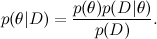
Here D is the data, what we know, and θ are the parameters of the model that we want to train. For example, in the SVD model, data are the ratings that users put on products, and the parameters of the model are factors that we train for users and products. - this is what we want to find, the probability distribution of the parameters of the model after we have taken into account the data; this is called posterior probability . This probability, as a rule, cannot be directly found, and this is precisely where Bayes theorem is needed.
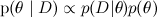
  - this is the so-called likelihood , the probability of the data, provided the model parameters are fixed; it is usually easy to find; in fact, the design of the model usually consists in setting the likelihood function. BUT
  - prior probability, it is a mathematical formalization of our intuition about the subject, a formalization of what we knew before, even before any experiments.
Thus, we come to one of the main tasks of Bayesian inference: to find the a posteriori distribution on hypotheses / parameters:
and find the maximum a posteriori hypothesis .
.
But if everything is so simple - they multiplied two functions, maximized the result - what is the whole science about? The problem is that the distributions that interest us are usually too complex to be maximized directly, analytically. There are too many variables in them, too complex connections between variables. But, on the other hand, they often have an additional structure that can be used, a structure in the form of independence ( ) and conditional independence (
  ) some variables.
Recall our conversation about naive Bayes : the model produced a very large number of parameters, and we made an additional assumption about the conditional independence of attributes (words) subject to the condition:

The result is a complex posterior distribution. managed to rewrite as

and in this form it turned out to be much easier to cope with (to train the parameters of each small distribution separately, and then choose v , which gives the maximum of the product). This is one of the simplest examples of decomposition (factorization) of a complex distribution into a product of simple ones. Today and in subsequent texts we will be able to generalize this method and bring it to unsurpassed heights.
So, let's look at one of the most convenient ways to represent large and complex probability distributions - Bayesian belief networks (Bayesian belief networks), which recently are often called simply directed graphical models (directed graphical models). A Bayesian network is a directed graph without directed cycles (this is a very important condition!), In which the vertices correspond to variables in the distribution, and the edges connect “connected” variables. Each node is assigned a conditional distribution of the node, provided its parents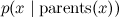 , and the Bayesian network graph means that a large joint distribution decomposes into a product of these conditional distributions.
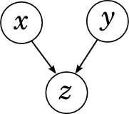
Here, for example, the graph corresponding to the naive Bayes:
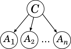
It corresponds to decomposition.

C has no ancestors, so we take its unconditional (marginal) distribution, and each of A i "grows" directly from C and is no longer connected with anyone.
We already know that in this case all the attributes A i are conditionally independent, provided that the category C is :

Let us now consider all the simplest variants of the Bayesian network and see what conditions of independence between variables they correspond to.
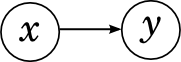
Let's start with a network of two variables, x and y . There are only two options: either there is no edge between x and y , or there is. If there is no edge, it simply means that x and y are independent, because such a graph corresponds to the decomposition .

And if there is an edge (let it go from x to y , it doesn't matter), we get the decomposition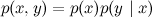 which literally by definition of conditional probability is always stupidly true for any distribution
  . Thus, a graph with two vertices with an edge does not give us new information.
Now go to the networks of the three variables, x , y and z . The easiest case is when there are no edges at all.
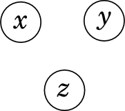
As with two variables, this means that x , y, and z are simply independent: .
.
Another simple case is when all edges are drawn between variables.
This case is also similar to the one discussed above; for example, let the edges go from x to y and z , and also from y to z . We get decomposition

which, again, is always true for any joint distribution . In this formula it would be possible to select variables in any order, nothing would change. Please note that directed loops in Bayesian networks are prohibited, and as a result, there are six options for how to draw all edges, not eight.
These observations, of course, are generalized to the case of any number of variables: if the variables are completely unrelated to each other, they are independent, and the graph in which all edges are drawn (with arrows in any direction, but so that directional cycles do not work) , corresponds to decomposition, which is always true, and does not give us any information.
In this section, we will look at three more interesting cases - these will be the “bricks” from which any Bayesian network can be made. Fortunately, it is enough to consider graphs in three variables - everything else will be generalized from them. In the examples below, I will somewhat sin against the truth and will intuitively interpret the edge, the arrow between the two variables, as “ x affects y ”, i.e. essentially as a causal relationship. In fact, this, of course, is not quite so - for example, you can often turn an edge without losing meaning (remember: in a column of two variables it did not matter in which direction the edge was drawn). And in general, this is a difficult philosophical question - what are "cause-effect relationships" and why are they needed? But for the reasoning on the fingers will come down.
Let's start with the serial communication between variables: x “affects” y , and y , in turn, “affects” z .
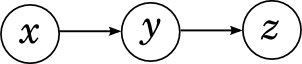
This graph represents the decomposition

Intuitively, this corresponds to a consistent causal relationship: if you run around in the winter without a hat, you will catch a cold, and if you catch a cold, your temperature will rise. It is obvious that x and y , as well as y and z are connected with each other, even the arrows are drawn directly between them. Are x and z interconnected in such a network, are these variables dependent? Of course! If you run in the winter without a hat, the likelihood of high temperatures rises. However, in such a network, x and z are connected only through y , and if we already know the value of y , x and z become independent: if you already know that you have caught a cold, it does not matter at all what caused it, the temperature will now rise (or not ) it is from a cold.
Formally, this corresponds to the conditional independence of x and z under the condition y ; let's check it out:

where the first equality is the definition of conditional probability, the second is our decomposition, and the third is the application of the Bayes theorem.
So, the consistent connection between the three variables tells us that the extreme variables are conditionally independent under the condition of the average. Everything is very logical and quite straightforward.
The next possible option is a diverging relationship: x “affects” both y and z .

This graph represents the decomposition

Intuitively, this corresponds to two consequences of the same reason: if you catch a cold, you may have a fever, and a cold can also begin. As in the previous case, it is obvious that x and y , as well as x and z are dependent, and the question is the relationship between y and z . Again, it is obvious that these variables are dependent: if you have a runny nose, this increases the likelihood that you have a cold, which means that the probability of a high temperature also rises.
However, in such a network, like in the previous case, y and z are connected only through x , and if we already know the meaning of the common cause, x , y and z become independent: if you already know that you have caught a cold, the cold and temperature become independent. Disclaimer: my medical examples are extremely conditional, in fact, I have no idea if runny nose and temperature are independent in life under the condition of a cold, and even I suspect that it is unlikely, because many other diseases can also cause both of these symptoms together. But in our conditional model in the universe there are no other illnesses besides the common cold.
Formally, this corresponds to the conditional independence of y and z under the condition x ; check it out even easier than serial communication:

So, the divergent relationship between the three variables tells us that the “consequences” are conditionally independent, provided that they have a “common cause”. If the reason is known, then the consequences become independent; as long as the cause is unknown, the effects through it are related. Again, while it seems to be nothing surprising.
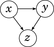
We have only one possible variant of the connection between the three variables: a convergent connection, when x and y together "influence" z .
The decomposition here turns out to be:

This is a situation in which the same effect may have two different causes: for example, the temperature may be the result of a cold, or maybe poisoning. Are cold and poisoning dependent? Not! In this situation, as long as the general effect is unknown, two reasons are not related to each other, and it is very easy to verify this formally:

However, if the “common effect” z becomes known, the situation changes. Now the common causes of a certain consequence begin to influence each other. This phenomenon is called “explaining away” in English: suppose you know that you have a fever. This greatly increases the likelihood of both colds and poisoning. However, if you now learn that you have been poisoned, the likelihood of a cold will decrease - the symptom "is already explained" by one of the possible causes, and the second becomes less likely.
Thus, with a converging connection, the two “causes” are independent, but only as long as the meaning of their “general effect” is unknown; if the general effect is signified, the causes become dependent.
But there is, as Vassily Ivanovich said, one nuance: when there is a converging link on the way, it is not enough to look only at its “general effect” in order to determine independence. In fact, even if there is no value for z , but one of its descendants has it (perhaps far enough), two reasons will still become dependent. Intuitively, this is also easy to understand: for example, suppose we do not observe the actual temperature, but observe its descendant - the thermometer readings. There probably are faulty thermometers in the world, so this is also some kind of probabilistic connection. However, observing the thermometer readings in the same way makes the common cold and poisoning dependent.
Sequential, converging and diverging connections are the three building blocks of which any acyclic directed graph consists. And our reasoning is quite enough to summarize the results on conditional dependence and independence on all such graphs. Of course, there is no time or place for formally proving general theorems, but the result is quite predictable - suppose you need to check in a large graph whether two vertices are independent (or even two sets of vertices). To do this, you look at all the paths in the graph (without taking into account the arrows) connecting these two sets of vertices. Each of these paths can be “broken” by one of the above constructions: for example, a sequential link will break if it has a meaning in the middle (the value of the variable is known), and a converging link will break if, on the contrary, there is no value (and not at the very top out of the way, nor in her descendants). If, as a result, all the paths are broken, then the sets of variables are truly independent; if not, no.
So, today we have considered a simple, convenient and important representation of factorizations of complex distributions - Bayesian networks. Next time we will look at another (but, of course, similar) graphical representation and begin to develop output algorithms, i.e. solving Bayesian inference problems in complex probabilistic models.
In order to move further and put these and many other methods into a common context, we need to develop some kind of common base, to learn the language spoken by modern data processing methods, the language of graphical probabilistic models . Today - the first part of this story, the most simple, with pictures and explanations.
')
Bayesian Output Tasks
First, let me briefly remind you of what we have already said . The main tool of machine learning is the Bayes theorem:
Here D is the data, what we know, and θ are the parameters of the model that we want to train. For example, in the SVD model, data are the ratings that users put on products, and the parameters of the model are factors that we train for users and products.
- this is what we want to find, the probability distribution of the parameters of the model after we have taken into account the data; this is called posterior probability . This probability, as a rule, cannot be directly found, and this is precisely where Bayes theorem is needed. - this is the so-called likelihood , the probability of the data, provided the model parameters are fixed; it is usually easy to find; in fact, the design of the model usually consists in setting the likelihood function. BUT - prior probability, it is a mathematical formalization of our intuition about the subject, a formalization of what we knew before, even before any experiments.Thus, we come to one of the main tasks of Bayesian inference: to find the a posteriori distribution on hypotheses / parameters:
and find the maximum a posteriori hypothesis
.Complexisation factorization and Bayesian networks
But if everything is so simple - they multiplied two functions, maximized the result - what is the whole science about? The problem is that the distributions that interest us are usually too complex to be maximized directly, analytically. There are too many variables in them, too complex connections between variables. But, on the other hand, they often have an additional structure that can be used, a structure in the form of independence (
) and conditional independence ( ) some variables.Recall our conversation about naive Bayes : the model produced a very large number of parameters, and we made an additional assumption about the conditional independence of attributes (words) subject to the condition:
The result is a complex posterior distribution.
managed to rewrite asand in this form it turned out to be much easier to cope with (to train the parameters of each small distribution separately, and then choose v , which gives the maximum of the product). This is one of the simplest examples of decomposition (factorization) of a complex distribution into a product of simple ones. Today and in subsequent texts we will be able to generalize this method and bring it to unsurpassed heights.
So, let's look at one of the most convenient ways to represent large and complex probability distributions - Bayesian belief networks (Bayesian belief networks), which recently are often called simply directed graphical models (directed graphical models). A Bayesian network is a directed graph without directed cycles (this is a very important condition!), In which the vertices correspond to variables in the distribution, and the edges connect “connected” variables. Each node is assigned a conditional distribution of the node, provided its parents
, and the Bayesian network graph means that a large joint distribution decomposes into a product of these conditional distributions.Here, for example, the graph corresponding to the naive Bayes:
It corresponds to decomposition.
C has no ancestors, so we take its unconditional (marginal) distribution, and each of A i "grows" directly from C and is no longer connected with anyone.
We already know that in this case all the attributes A i are conditionally independent, provided that the category C is :
Let us now consider all the simplest variants of the Bayesian network and see what conditions of independence between variables they correspond to.
Bayesian networks with two and three variables: trivial cases
Let's start with a network of two variables, x and y . There are only two options: either there is no edge between x and y , or there is. If there is no edge, it simply means that x and y are independent, because such a graph corresponds to the decomposition
.And if there is an edge (let it go from x to y , it doesn't matter), we get the decomposition
which literally by definition of conditional probability is always stupidly true for any distribution . Thus, a graph with two vertices with an edge does not give us new information.Now go to the networks of the three variables, x , y and z . The easiest case is when there are no edges at all.
As with two variables, this means that x , y, and z are simply independent:
.Another simple case is when all edges are drawn between variables.
This case is also similar to the one discussed above; for example, let the edges go from x to y and z , and also from y to z . We get decomposition
which, again, is always true for any joint distribution
. In this formula it would be possible to select variables in any order, nothing would change. Please note that directed loops in Bayesian networks are prohibited, and as a result, there are six options for how to draw all edges, not eight.These observations, of course, are generalized to the case of any number of variables: if the variables are completely unrelated to each other, they are independent, and the graph in which all edges are drawn (with arrows in any direction, but so that directional cycles do not work) , corresponds to decomposition, which is always true, and does not give us any information.
Bayesian networks with three variables: interesting cases
In this section, we will look at three more interesting cases - these will be the “bricks” from which any Bayesian network can be made. Fortunately, it is enough to consider graphs in three variables - everything else will be generalized from them. In the examples below, I will somewhat sin against the truth and will intuitively interpret the edge, the arrow between the two variables, as “ x affects y ”, i.e. essentially as a causal relationship. In fact, this, of course, is not quite so - for example, you can often turn an edge without losing meaning (remember: in a column of two variables it did not matter in which direction the edge was drawn). And in general, this is a difficult philosophical question - what are "cause-effect relationships" and why are they needed? But for the reasoning on the fingers will come down.
Serial communication
Let's start with the serial communication between variables: x “affects” y , and y , in turn, “affects” z .
This graph represents the decomposition
Intuitively, this corresponds to a consistent causal relationship: if you run around in the winter without a hat, you will catch a cold, and if you catch a cold, your temperature will rise. It is obvious that x and y , as well as y and z are connected with each other, even the arrows are drawn directly between them. Are x and z interconnected in such a network, are these variables dependent? Of course! If you run in the winter without a hat, the likelihood of high temperatures rises. However, in such a network, x and z are connected only through y , and if we already know the value of y , x and z become independent: if you already know that you have caught a cold, it does not matter at all what caused it, the temperature will now rise (or not ) it is from a cold.
Formally, this corresponds to the conditional independence of x and z under the condition y ; let's check it out:
where the first equality is the definition of conditional probability, the second is our decomposition, and the third is the application of the Bayes theorem.
So, the consistent connection between the three variables tells us that the extreme variables are conditionally independent under the condition of the average. Everything is very logical and quite straightforward.
Divergent link
The next possible option is a diverging relationship: x “affects” both y and z .
This graph represents the decomposition
Intuitively, this corresponds to two consequences of the same reason: if you catch a cold, you may have a fever, and a cold can also begin. As in the previous case, it is obvious that x and y , as well as x and z are dependent, and the question is the relationship between y and z . Again, it is obvious that these variables are dependent: if you have a runny nose, this increases the likelihood that you have a cold, which means that the probability of a high temperature also rises.
However, in such a network, like in the previous case, y and z are connected only through x , and if we already know the meaning of the common cause, x , y and z become independent: if you already know that you have caught a cold, the cold and temperature become independent. Disclaimer: my medical examples are extremely conditional, in fact, I have no idea if runny nose and temperature are independent in life under the condition of a cold, and even I suspect that it is unlikely, because many other diseases can also cause both of these symptoms together. But in our conditional model in the universe there are no other illnesses besides the common cold.
Formally, this corresponds to the conditional independence of y and z under the condition x ; check it out even easier than serial communication:
So, the divergent relationship between the three variables tells us that the “consequences” are conditionally independent, provided that they have a “common cause”. If the reason is known, then the consequences become independent; as long as the cause is unknown, the effects through it are related. Again, while it seems to be nothing surprising.
Converging relationship
We have only one possible variant of the connection between the three variables: a convergent connection, when x and y together "influence" z .
The decomposition here turns out to be:
This is a situation in which the same effect may have two different causes: for example, the temperature may be the result of a cold, or maybe poisoning. Are cold and poisoning dependent? Not! In this situation, as long as the general effect is unknown, two reasons are not related to each other, and it is very easy to verify this formally:
However, if the “common effect” z becomes known, the situation changes. Now the common causes of a certain consequence begin to influence each other. This phenomenon is called “explaining away” in English: suppose you know that you have a fever. This greatly increases the likelihood of both colds and poisoning. However, if you now learn that you have been poisoned, the likelihood of a cold will decrease - the symptom "is already explained" by one of the possible causes, and the second becomes less likely.
Thus, with a converging connection, the two “causes” are independent, but only as long as the meaning of their “general effect” is unknown; if the general effect is signified, the causes become dependent.
But there is, as Vassily Ivanovich said, one nuance: when there is a converging link on the way, it is not enough to look only at its “general effect” in order to determine independence. In fact, even if there is no value for z , but one of its descendants has it (perhaps far enough), two reasons will still become dependent. Intuitively, this is also easy to understand: for example, suppose we do not observe the actual temperature, but observe its descendant - the thermometer readings. There probably are faulty thermometers in the world, so this is also some kind of probabilistic connection. However, observing the thermometer readings in the same way makes the common cold and poisoning dependent.
Putting it all together
Sequential, converging and diverging connections are the three building blocks of which any acyclic directed graph consists. And our reasoning is quite enough to summarize the results on conditional dependence and independence on all such graphs. Of course, there is no time or place for formally proving general theorems, but the result is quite predictable - suppose you need to check in a large graph whether two vertices are independent (or even two sets of vertices). To do this, you look at all the paths in the graph (without taking into account the arrows) connecting these two sets of vertices. Each of these paths can be “broken” by one of the above constructions: for example, a sequential link will break if it has a meaning in the middle (the value of the variable is known), and a converging link will break if, on the contrary, there is no value (and not at the very top out of the way, nor in her descendants). If, as a result, all the paths are broken, then the sets of variables are truly independent; if not, no.
So, today we have considered a simple, convenient and important representation of factorizations of complex distributions - Bayesian networks. Next time we will look at another (but, of course, similar) graphical representation and begin to develop output algorithms, i.e. solving Bayesian inference problems in complex probabilistic models.
Source: https://habr.com/ru/post/176461/
All Articles