Regularization in a limited Boltzmann machine, experiment

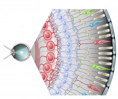Hey. In this post we will conduct an experiment in which we test two types of regularization in a limited Boltzmann machine . As it turned out, RBM is very sensitive to model parameters, such as the moment and local field of a neuron (for more information about all parameters, see Jeffrey Hinton’s RBM Practical Guide ). But for a complete picture and for getting patterns like these , I lacked one more parameter - regularization. The limited Boltzmann machines can be treated as a variety of the Markov network, and as another neural network, but if you dig deeper, you will see an analogy with vision. Like the primary visual cortex , which receives information from the retina through the optic nerve (forgive me to biologists for such a simplification), RBM searches for simple patterns in the input image. The analogy does not end there, if we interpret the very small and zero weights as the absence of weight, then we get that each hidden neuron RBM forms a certain receptive field , and a deep network formed from RBM trained forms simple images from simple images; in principle, the visual cortex deals with something similar, although it’s probably more complicated =)

L1 and L2 regularization

We begin, perhaps, with a brief description of what model regularization is - a way to impose a penalty on the objective function for the complexity of the model. From Bayesian point of view, this is a way to take into account some a priori information about the distribution of model parameters. An important feature is that regularization helps to avoid retraining the model. Denote the model parameters as θ = {θ_i}, i = 1..n. The final objective function is C = η (E + λR) , where E is the main objective function of the model, R = R (θ) is a function of the parameters of the model, this and lambda are the learning rate and the regularization parameter, respectively. Thus, to calculate the gradient of the final objective function, it will be necessary to calculate the gradient of the regularization function:
')


We consider two types of regularization whose roots are in the Lp metric . The regularization function of L1 and its derivatives are as follows:





L2 regularization is as follows:





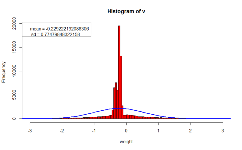
Both regularization methods penalize the model for a large value of weights, in the first case with absolute weights, in the second with squares of weights, thus, the distribution of weights will approach normal with a center at zero and a large peak. A more detailed comparison of L1 and L2 can be found here . As we will see later, about 70% of the weights will be less than 10 ^ (- 8).

RBM Regularization

The day before last, I described an example of implementing RBM in C # . I will rely on the same implementation to show where the regularization is embedded, but first the formulas. The goal of learning RBM is to maximize the likelihood that the restored image will be identical to the input one:



Generally speaking, the algorithm maximizes the logarithm of probability, and in order to introduce a penalty, it is necessary to subtract the value of the regularization function from the obtained probability, as a result, the new objective function takes the following form:



The derivative of such a function by parameter will look like this:



The contrastive divergence algorithm consists of a positive phase and a negative one, thus, in order to add regularization, it is sufficient to subtract the value of the derivative of the regularization function from the value of the positive phase, after subtracting the negative phase:



Go to the experiments. The same data set was used as test data as in the previous post . In all cases, training was conducted exactly 1000 epochs. I will give two ways to visualize the patterns found, in the first case (drawing in gray tones) the dark value corresponds to the minimum value of the weight, and the white to the maximum; in the second drawing, black corresponds to zero, an increase in the red component corresponds to an increase in a positive direction, and an increase in the blue component - in a negative one. I will also give a histogram of the distribution of weights and small comments.

Without regularization

• error value on the training set: 0.188181367765024
• error value on the cross qualification set: 21.0910315518859

The templates turned out very blurry and difficult to analyze. The average value of the scales is shifted to the left, and the absolute value of the scales reaches 2 or more.

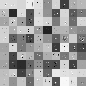
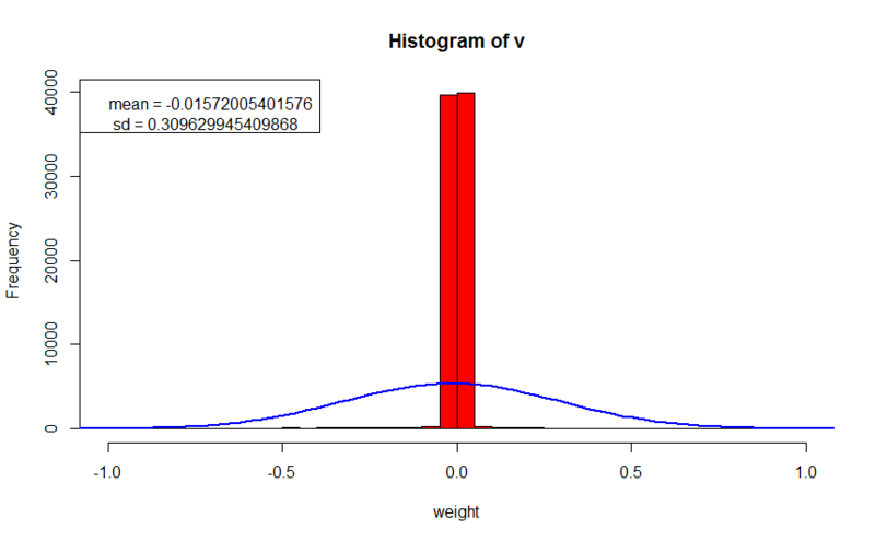
L2 regularization

• error value on the training set: 10.1198906337165
• error value at cross qualification set: 23.3600809429977
• regularization parameter: 0.1

Here we see clearer images. We can already discern that in some images some peculiarities of letters are really taken into account. Despite the fact that the error on the training set is 100 times worse than when learning without regularization, the error on the cross-qualification set does not much exceed the first experiment, which suggests that the generalizing ability of the network on unfamiliar images did not deteriorate much (it should be noted that the error calculation did not include the value of the regularization function, which allows us to compare values ​​with previous experience). The weights are concentrated around zero, and not much higher than 0.2 in absolute value, which is 10 times less than in previous experience.

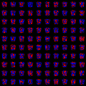
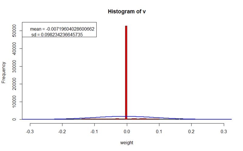
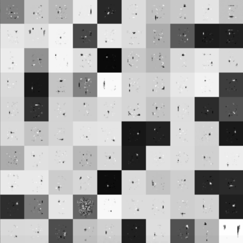
L1 regularization

• error value on the training set: 4.42672814826447
• error value on the cross qualification set: 17.3700437102876
• regularization parameter: 0.005

In this experience, we see clear patterns, and especially receptive fields (around the blue-red spots, all weights are almost zero). Patterns can even be analyzed, we can see, for example, edges from W (the first row is the fourth picture), or a pattern that reflects the average size of the input images (in the fifth row 8 and 10 pictures). The recovery error on the training set is 40 times worse than in the first experiment, but better than with L2 regularization, at the same time the error on the unknown set is better than in both previous experiments, which indicates an even better generalizing ability. Weights are also concentrated around zero, and in most cases do not exceed it much. The significant difference in the regularization parameter is explained by the fact that when calculating the gradient for L2, the parameter is multiplied by the weight value, as a rule, these two numbers are less than 1; but with L1, the parameter is multiplied by | 1 |, and the final value will be of the same order as the regularization parameter.

Conclusion

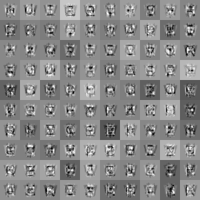
As a conclusion, I would like to say that the BSR is really a very sensitive thing to the parameters. And the main thing is not to break down in the process of finding a solution -) In the end, I’ll give an increased representation of one of the RBM trainers with L1 regularization, but already for 5000 epochs.


UPDATE :
I recently trained rbm on a full set of capital letters 4 fonts of 3 styles, during 5000 iterations with L1 regularization, it took about 14 hours, but the result is even more interesting, the features turned out to be even more local and clean