Evaluation of algorithms complexity

Introduction

For any programmer, it is important to know the basics of the theory of algorithms, since it is this science that studies the general characteristics of algorithms and the formal models of their presentation. Even from computer science lessons, we are taught to make flowcharts, which, in turn, helps in writing more complex tasks than in school. It is also not a secret that there are almost always several ways to solve a particular task: some suggest spending a lot of time, other resources, and still others only help to find a solution.

You should always look for the optimum in accordance with the task, in particular, when developing algorithms for solving a class of problems.
It is also important to evaluate how the algorithm will behave with the initial values ​​of different volumes and quantities, what resources it will need and how long it will take to output the final result.
This is the topic of the theory of algorithms - the theory of asymptotic analysis of algorithms.

I propose in this article to describe the main evaluation criteria and give an example of the evaluation of the simplest algorithm. On Habrahabr there is already an article about methods for evaluating algorithms, but it focuses mainly on high school students. This publication can be considered a deepening of that article.
')

Definitions

The main indicator of the complexity of the algorithm is the time required to solve the problem and the amount of required memory.
Also, when analyzing the complexity for a class of tasks, a certain number is defined that characterizes a certain amount of data - the size of the input .
So, we can conclude that the complexity of the algorithm is a function of the size of the input.
The complexity of the algorithm may be different for the same input size, but different input data.

There are notions of complexity at worst , average or best . Usually, the complexity is evaluated at worst.

In the worst case, the time complexity is a function of the size of the input, equal to the maximum number of operations performed during the operation of the algorithm in solving the problem of a given size.
In the worst case, capacitive complexity is a function of the size of the input, equal to the maximum number of memory cells that were addressed when solving problems of a given size.

Order of increase in complexity of algorithms

The order of growth of complexity (or axiomatic complexity) describes the approximate behavior of the complexity function of an algorithm with a large input size. From this it follows that in assessing the time complexity there is no need to consider elementary operations, it suffices to consider the steps of the algorithm.

An algorithm step is a set of sequential elementary operations whose execution time does not depend on the size of the input, that is, is bounded above by some constant.

Types of asymptotic estimates

O - score for the worst case.

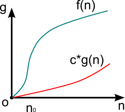
Consider the complexity f (n)> 0 , the function of the same order g (n)> 0 , the input size n> 0 .
If f (n) = O (g (n)) and there are constants c> 0 , n ₀ > 0 , then
0 <f (n) <c * g (n),
for n> n ₀ .



The function g (n) in this case is the asymptotic-exact estimate f (n). If f (n) is the complexity function of the algorithm, then the complexity order is defined as f (n) - O (g (n)).

This expression defines a class of functions that do not grow faster than g (n) up to a constant factor.

Examples of asymptotic functions

f (n)	g (n)
2n 2 + 7n - 3	n 2
98n * ln (n)	n * ln (n)
5n + 2	n
eight	one

Ω - score for the best case

The definition is similar to the worst case definition, however
f (n) = Ω (g (n)) if
0 <c * g (n) <f (n)



Ω (g (n)) defines a class of functions that do not grow more slowly than the function g (n) up to a constant factor.

Θ - estimate for the average case

It is only worth mentioning that in this case the function f (n) with n> n ₀ everywhere is between c ₁ * g (n) and c ₂ * g (n) , where c is a constant factor.
For example, with f (n) = n ² + n ; g (n) = n ² .

Criteria for assessing the complexity of algorithms

Uniform weight criterion (RVK) assumes that each step of the algorithm is executed for one unit of time, and a memory cell for one unit of volume (with accuracy to a constant).
The logarithmic weight criterion (LVK) takes into account the size of the operand that is processed by an operation and the value stored in the memory cell.


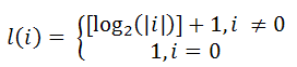
The time complexity in LVD is determined by the value of l (O _p ) , where O _p is the value of the operand.
Capacitive complexity in LVD is determined by the value of l (M) , where M is the value of the memory cell.

An example of an estimate of the difficulty in calculating factorial

It is necessary to analyze the complexity of the algorithm for calculating factorial. To do this, we write this task in the pseudocode of the C language:

void main() { int result = 1; int i; const n = ...; for (i = 2; i <= n; i++) result = result * n; } 

Temporary complexity with uniform weight criteria

It is enough just to determine that the input size of this task is n .
The number of steps is (n - 1) .

Thus, the time complexity with RVK is O (n) .

Time complexity with log weight criterion

In this paragraph, we should highlight the operations that need to be assessed. First, these are comparison operations. Secondly, the operations of changing variables (addition, multiplication). Assignment operations are not taken into account, as it is assumed to be instantaneous.

So, in this task there are three operations:

1) i <= n

At the ith step, log (n) is obtained.
Since steps (n-1) , the complexity of this operation will be (n-1) * log (n) .

2) i = i + 1

At the ith step, log (i) is obtained.
Thus, the result is .

3) result = result * i

At the i-th step log ((i-1)!) .
Thus, the result is .

If we add up all the resulting values ​​and discard the terms, which obviously grow slower with increasing n , we get the final expression .

Capacitive complexity with uniform weight criteria

Everything is simple here. It is necessary to count the number of variables. If arrays are used in the task, each cell of the array is considered as a variable.
Since the number of variables does not depend on the size of the input, the complexity will be equal to O (1) .

Capacitive complexity with a logarithmic weight criterion

In this case, consider the maximum value that can be in the memory cell. If the value is not defined (for example, with the operand i> 10), then it is considered that there is some limiting value V _max .
In this task, there is a variable whose value does not exceed n (i) , and a variable whose value does not exceed n! (result) . Thus, the estimate is O (log (n!)) .

findings

Studying the complexity of algorithms is quite an exciting task. At the moment, the analysis of the simplest algorithms is included in the curricula of technical specialties (to be precise, of the generalized “Computer Science and Computing Technology” direction) involved in computer science and applied mathematics in the field of IT.
Based on complexity, different classes of tasks are distinguished: P , NP , NPC . But this is no longer a problem in the theory of asymptotic analysis of algorithms.