Data preprocessing and model analysis
Hello. In the last post I talked about some basic classification methods. Today, due to the specifics of the last house, the post will be not so much about the methods themselves, as about data processing and analysis of the models obtained.
The data was provided by the Department of Statistics of the University of Munich. Here you can take a dataset itself, as well as the description of the data itself (the names of the fields are given in German). The data collected loan applications, where each application is described by 20 variables. In addition, each application corresponds to whether the applicant has been given a loan or not. Here you can see in detail what of the variables means.
')
Our task was to build a model that would predict a decision to be made on one or another applicant.

Alas, there were no test data and systems for testing our models, as, for example, it was done in MNIST . In this regard, we had some room for imagination in terms of the validation of our models.
Let's first take a look at the data itself. The following graph shows the histograms of the distributions of all available variables. The order of occurrence of variables is specifically modified for clarity.


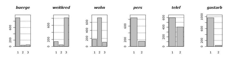
Looking at these graphs, we can draw several conclusions. First, most of the variables are categorical in fact, that is, they take only a couple (pair) of values. Secondly, there are only two (well, maybe three) conditionally continuous variables, namely, hoehe and alter . Third, there are no emissions.
When working with continuous variables, generally speaking, you can pretty much forgive the mind of their distribution. For example, multimodality, when the density has a strange hilly shape, with several peaks. Something similar can be seen on the density graph of the laufzeit variable. But the extended tails of the distributions are the main headache in the construction of models, since they very strongly influence their properties and appearance. Emissions also greatly affect the quality of the models built, but since we are lucky and we don’t have them, I’ll tell you about the emissions some time next.
Returning to our tails, the variables hoehe and alter have one feature: they are not normal. Ie, they are very similar to lognormal, due to the strong right tail. Considering all the above, we have some reason to recologize these variables in order to tighten these tails.
What is the strength in, brother? Or who are all these
Often, when analyzing, some variables are unnecessary. That is, well, absolutely. This means that if we throw them out of the analysis, then in solving our problem, we will lose almost nothing even in the worst case. In our case of credit scoring, by losses we mean a slightly decreased classification accuracy.
This is what will happen in the worst case. However, practice shows that with careful selection of variables, popularly known as feature selection , you can even win exactly. Insignificant variables introduce noise exclusively into the model, with almost no effect on the result. And when they are collected quite a lot, we have to separate the wheat from the chaff.
In practice, this task arises from the fact that by the time of data collection, experts do not yet know which variables will be most significant in the analysis. At the same time, during the experiment itself and data collection, no one bothers the experimenters to collect all the variables that can be collected at all. They say that we will collect all that is, and analysts will somehow sort it out themselves.
Cutting variables must be wisely. If we simply cut the data on the frequency of occurrence of a trait, for example, in the case of the gastarb variable, then we cannot guarantee that we will not discard a very significant trait. In some textual or biological data, this problem is even more pronounced, since there are very rarely any variables that take on non-zero values.
The problem with the selection of signs is that for each model, tied to the data, the criterion for the selection of signs will be its own, specially built for this model. For example, for linear models, t-statistics on the significance of the coefficients are used , and for Random Forest - the relative importance of variables in the cascade of trees . And sometimes feature selection can generally be explicitly built into the model .
For simplicity, consider only the significance of variables in a linear model. We simply construct a generalized linear model, GLM. Since our target variable is a class label, it therefore has (conditionally) a binomial distribution. Using the function glm in R, we construct this model and look under the hood for it, calling a summary for it. As a result, we get the following label:

We are interested in the very last column. This column indicates the probability that our coefficient is zero, that is, it does not play a role in the final model. The asterisks here indicate the relative significance of the coefficients. From the table we see that, generally speaking, we can ruthlessly cut out almost all variables, except laufkont , laufzeit , moral and sparkont ( intercept is the shift parameter, we also need it). We chose them on the basis of the statistics obtained, that is, those variables for which the statistics for “departure” is less than or equal to 0.01.
If you close your eyes to the validation of the model, assuming that the linear model does not overtake our data, you can check the validity of our hypothesis. Namely, we will test the accuracy of two models on all data: a model with 4 variables and a model with 20. For 20 variables, the classification accuracy will be 77.1%, while for a model with 4 variables, 76.1%. As you can see, not very sorry.
It is interesting that the variables we predicted do not affect the model in any way. Being never prologized and prologicized twice, they did not reach even 0.1.
We decided to build the classifiers in Python using Scikit. In the analysis, we decided to use all the main classifiers that scikit provides, having played with their hyperparameters. Here is a list of what was launched:
At the end of the article - links to the documentation for classes that implement these algorithms.
Since we did not have the opportunity to test the output explicitly, we used the cross-validation method. We took 10 as the number of folds. As a result, we derive the average value of the classification accuracy from all 10 folds.
The implementation is very transparent.
After we launched our script, we got the following results:
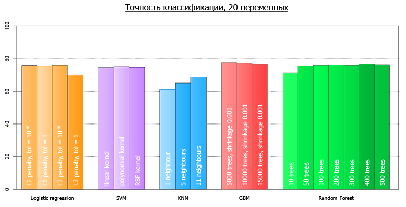
More clearly, they can be visualized as follows:
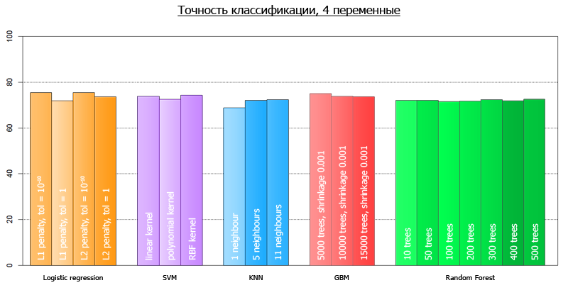
The average accuracy for all models on 4 variables is 72.7
The average accuracy for all models on all-all variables is 73.7
The discrepancy with the ones predicted at the beginning of the article is explained by the fact that those tests were performed on a different framework.
Looking at the results of the accuracy of the models we obtained, we can draw a couple of interesting conclusions. We built a stack of different models, linear and nonlinear. As a result, all these models show approximately the same accuracy on the data. That is, such models as RF and SVM did not give significant advantages in accuracy in comparison with the linear model. This is most likely a consequence of the fact that the original data is almost certainly some kind of linear relationship and was generated.
The consequence of this is that it is pointless to chase these data for accuracy using complex massive methods, such as Random Forest, SVM or Gradient Boosting. That is, everything that could be caught in this data was already caught by the linear model. Otherwise, if there are explicit non-linear dependencies in the data, this difference in accuracy would be more significant.
This tells us that sometimes the data is not as complex as it seems, and very quickly you can come to the actual maximum of what can be squeezed out of them.
Moreover, out of the highly abbreviated data through the use of feature selection, our accuracy did not actually suffer. Ie our solution for this data was not only simple (cheaply), but also compact.
Logistic Regression (our GLM case)
SVM
kNN
Random forest
Gradient boosting
In addition, here is an example of working with cross-validation.
For help in writing an article thanks to the Data Mining track from GameChangers , as well as Alexey Natyokin.
Task
The data was provided by the Department of Statistics of the University of Munich. Here you can take a dataset itself, as well as the description of the data itself (the names of the fields are given in German). The data collected loan applications, where each application is described by 20 variables. In addition, each application corresponds to whether the applicant has been given a loan or not. Here you can see in detail what of the variables means.
')
Our task was to build a model that would predict a decision to be made on one or another applicant.
Alas, there were no test data and systems for testing our models, as, for example, it was done in MNIST . In this regard, we had some room for imagination in terms of the validation of our models.
Pre-processing of data
Let's first take a look at the data itself. The following graph shows the histograms of the distributions of all available variables. The order of occurrence of variables is specifically modified for clarity.
Looking at these graphs, we can draw several conclusions. First, most of the variables are categorical in fact, that is, they take only a couple (pair) of values. Secondly, there are only two (well, maybe three) conditionally continuous variables, namely, hoehe and alter . Third, there are no emissions.
When working with continuous variables, generally speaking, you can pretty much forgive the mind of their distribution. For example, multimodality, when the density has a strange hilly shape, with several peaks. Something similar can be seen on the density graph of the laufzeit variable. But the extended tails of the distributions are the main headache in the construction of models, since they very strongly influence their properties and appearance. Emissions also greatly affect the quality of the models built, but since we are lucky and we don’t have them, I’ll tell you about the emissions some time next.
Returning to our tails, the variables hoehe and alter have one feature: they are not normal. Ie, they are very similar to lognormal, due to the strong right tail. Considering all the above, we have some reason to recologize these variables in order to tighten these tails.
What is the strength in, brother? Or who are all these people variable?
Often, when analyzing, some variables are unnecessary. That is, well, absolutely. This means that if we throw them out of the analysis, then in solving our problem, we will lose almost nothing even in the worst case. In our case of credit scoring, by losses we mean a slightly decreased classification accuracy.
This is what will happen in the worst case. However, practice shows that with careful selection of variables, popularly known as feature selection , you can even win exactly. Insignificant variables introduce noise exclusively into the model, with almost no effect on the result. And when they are collected quite a lot, we have to separate the wheat from the chaff.
In practice, this task arises from the fact that by the time of data collection, experts do not yet know which variables will be most significant in the analysis. At the same time, during the experiment itself and data collection, no one bothers the experimenters to collect all the variables that can be collected at all. They say that we will collect all that is, and analysts will somehow sort it out themselves.
Cutting variables must be wisely. If we simply cut the data on the frequency of occurrence of a trait, for example, in the case of the gastarb variable, then we cannot guarantee that we will not discard a very significant trait. In some textual or biological data, this problem is even more pronounced, since there are very rarely any variables that take on non-zero values.
The problem with the selection of signs is that for each model, tied to the data, the criterion for the selection of signs will be its own, specially built for this model. For example, for linear models, t-statistics on the significance of the coefficients are used , and for Random Forest - the relative importance of variables in the cascade of trees . And sometimes feature selection can generally be explicitly built into the model .
For simplicity, consider only the significance of variables in a linear model. We simply construct a generalized linear model, GLM. Since our target variable is a class label, it therefore has (conditionally) a binomial distribution. Using the function glm in R, we construct this model and look under the hood for it, calling a summary for it. As a result, we get the following label:
We are interested in the very last column. This column indicates the probability that our coefficient is zero, that is, it does not play a role in the final model. The asterisks here indicate the relative significance of the coefficients. From the table we see that, generally speaking, we can ruthlessly cut out almost all variables, except laufkont , laufzeit , moral and sparkont ( intercept is the shift parameter, we also need it). We chose them on the basis of the statistics obtained, that is, those variables for which the statistics for “departure” is less than or equal to 0.01.
If you close your eyes to the validation of the model, assuming that the linear model does not overtake our data, you can check the validity of our hypothesis. Namely, we will test the accuracy of two models on all data: a model with 4 variables and a model with 20. For 20 variables, the classification accuracy will be 77.1%, while for a model with 4 variables, 76.1%. As you can see, not very sorry.
It is interesting that the variables we predicted do not affect the model in any way. Being never prologized and prologicized twice, they did not reach even 0.1.
Analysis
We decided to build the classifiers in Python using Scikit. In the analysis, we decided to use all the main classifiers that scikit provides, having played with their hyperparameters. Here is a list of what was launched:
At the end of the article - links to the documentation for classes that implement these algorithms.
Since we did not have the opportunity to test the output explicitly, we used the cross-validation method. We took 10 as the number of folds. As a result, we derive the average value of the classification accuracy from all 10 folds.
The implementation is very transparent.
View code
from sklearn.externals import joblib from sklearn import cross_validation from sklearn import svm from sklearn import neighbors from sklearn.ensemble import GradientBoostingClassifier from sklearn.ensemble import RandomForestClassifier from sklearn.linear_model import LogisticRegression import numpy as np def avg(x): s = 0.0 for t in x: s += t return (s/len(x))*100.0 dataset = joblib.load('kredit.pkl') # , target = [x[0] for x in dataset] target = np.array(target) train = [x[1:] for x in dataset] numcv = 10 # glm = LogisticRegression(penalty='l1', tol=1) scores = cross_validation.cross_val_score(glm, train, target, cv = numcv) print("Logistic Regression with L1 metric - " + ' avg = ' + ('%2.1f'%avg(scores))) linSVM = svm.SVC(kernel='linear', C=1) scores = cross_validation.cross_val_score(linSVM, train, target, cv = numcv) print("SVM with linear kernel - " + ' avg = ' + ('%2.1f'%avg(scores))) poly2SVM = svm.SVC(kernel='poly', degree=2, C=1) scores = cross_validation.cross_val_score(poly2SVM, train, target, cv = numcv) print("SVM with polynomial kernel degree 2 - " + ' avg = ' + ('%2.1f' % avg(scores))) rbfSVM = svm.SVC(kernel='rbf', C=1) scores = cross_validation.cross_val_score(rbfSVM, train, target, cv = numcv) print("SVM with rbf kernel - " + ' avg = ' + ('%2.1f'%avg(scores))) knn = neighbors.KNeighborsClassifier(n_neighbors = 1, weights='uniform') scores = cross_validation.cross_val_score(knn, train, target, cv = numcv) print("kNN 1 neighbour - " + ' avg = ' + ('%2.1f'%avg(scores))) knn = neighbors.KNeighborsClassifier(n_neighbors = 5, weights='uniform') scores = cross_validation.cross_val_score(knn, train, target, cv = numcv) print("kNN 5 neighbours - " + ' avg = ' + ('%2.1f'%avg(scores))) knn = neighbors.KNeighborsClassifier(n_neighbors = 11, weights='uniform') scores = cross_validation.cross_val_score(knn, train, target, cv = numcv) print("kNN 11 neighbours - " + ' avg = ' + ('%2.1f'%avg(scores))) gbm = GradientBoostingClassifier(learning_rate = 0.001, n_estimators = 5000) scores = cross_validation.cross_val_score(gbm, train, target, cv = numcv) print("Gradient Boosting 5000 trees, shrinkage 0.001 - " + ' avg = ' + ('%2.1f'%avg(scores))) gbm = GradientBoostingClassifier(learning_rate = 0.001, n_estimators = 10000) scores = cross_validation.cross_val_score(gbm, train, target, cv = numcv) print("Gradient Boosting 10000 trees, shrinkage 0.001 - " + ' avg = ' + ('%2.1f'%avg(scores))) gbm = GradientBoostingClassifier(learning_rate = 0.001, n_estimators = 15000) scores = cross_validation.cross_val_score(gbm, train, target, cv = numcv) print("Gradient Boosting 15000 trees, shrinkage 0.001 - " + ' avg = ' + ('%2.1f'%avg(scores))) # - forest = RandomForestClassifier(n_estimators = 10, n_jobs = 1) scores = cross_validation.cross_val_score(forest, train, target, cv=numcv) print("Random Forest 10 - " +' avg = ' + ('%2.1f'%avg(scores))) forest = RandomForestClassifier(n_estimators = 50, n_jobs = 1) scores = cross_validation.cross_val_score(forest, train, target, cv=numcv) print("Random Forest 50 - " +' avg = ' + ('%2.1f'%avg(scores))) forest = RandomForestClassifier(n_estimators = 100, n_jobs = 1) scores = cross_validation.cross_val_score(forest, train, target, cv=numcv) print("Random Forest 100 - " +' avg = '+ ('%2.1f'%avg(scores))) forest = RandomForestClassifier(n_estimators = 200, n_jobs = 1) scores = cross_validation.cross_val_score(forest, train, target, cv=numcv) print("Random Forest 200 - " +' avg = ' + ('%2.1f'%avg(scores))) forest = RandomForestClassifier(n_estimators = 300, n_jobs = 1) scores = cross_validation.cross_val_score(forest, train, target, cv=numcv) print("Random Forest 300 - " +' avg = '+ ('%2.1f'%avg(scores))) forest = RandomForestClassifier(n_estimators = 400, n_jobs = 1) scores = cross_validation.cross_val_score(forest, train, target, cv=numcv) print("Random Forest 400 - " +' avg = '+ ('%2.1f'%avg(scores))) forest = RandomForestClassifier(n_estimators = 500, n_jobs = 1) scores = cross_validation.cross_val_score(forest, train, target, cv=numcv) print("Random Forest 500 - " +' avg = '+ ('%2.1f'%avg(scores))) After we launched our script, we got the following results:
| Method with parameters | Average accuracy on 4 variables | Average accuracy on 20 variables |
|---|---|---|
| Logistic Regression, L1 metric | 75.5 | 75.2 |
| SVM with linear kernel | 73.9 | 74.4 |
| SVM with polynomial kernel | 72.6 | 74.9 |
| SVM with rbf kernel | 74.3 | 74.7 |
| kNN 1 neighbor | 68.8 | 61.4 |
| kNN 5 neighbors | 72.1 | 65.1 |
| kNN 11 neighbors | 72.3 | 68.7 |
| Gradient Boosting 5000 trees shrinkage 0.001 | 75.0 | 77.6 |
| Gradient Boosting 10000 trees shrinkage 0.001 | 73.8 | 77.2 |
| Gradient Boosting 15000 trees shrinkage 0.001 | 73.7 | 76.5 |
| Random Forest 10 | 72.0 | 71.2 |
| Random Forest 50 | 72.1 | 75.5 |
| Random Forest 100 | 71.6 | 75.9 |
| Random Forest 200 | 71.8 | 76.1 |
| Radom Forest 300 | 72.4 | 75.9 |
| Random Forest 400 | 71.9 | 76.7 |
| Random Forest 500 | 72.6 | 76.2 |
More clearly, they can be visualized as follows:
The average accuracy for all models on 4 variables is 72.7
The average accuracy for all models on all-all variables is 73.7
The discrepancy with the ones predicted at the beginning of the article is explained by the fact that those tests were performed on a different framework.
findings
Looking at the results of the accuracy of the models we obtained, we can draw a couple of interesting conclusions. We built a stack of different models, linear and nonlinear. As a result, all these models show approximately the same accuracy on the data. That is, such models as RF and SVM did not give significant advantages in accuracy in comparison with the linear model. This is most likely a consequence of the fact that the original data is almost certainly some kind of linear relationship and was generated.
The consequence of this is that it is pointless to chase these data for accuracy using complex massive methods, such as Random Forest, SVM or Gradient Boosting. That is, everything that could be caught in this data was already caught by the linear model. Otherwise, if there are explicit non-linear dependencies in the data, this difference in accuracy would be more significant.
This tells us that sometimes the data is not as complex as it seems, and very quickly you can come to the actual maximum of what can be squeezed out of them.
Moreover, out of the highly abbreviated data through the use of feature selection, our accuracy did not actually suffer. Ie our solution for this data was not only simple (cheaply), but also compact.
Documentation
Logistic Regression (our GLM case)
SVM
kNN
Random forest
Gradient boosting
In addition, here is an example of working with cross-validation.
For help in writing an article thanks to the Data Mining track from GameChangers , as well as Alexey Natyokin.
Source: https://habr.com/ru/post/173049/
All Articles