Building a system for optical recognition of structural information on the example of Imago OCR

In this article I will talk about how you can build an optical recognition system for structural information, based on the algorithms used in image processing and their implementation within the OpenCV library. Behind the description of the system is an actively developing open source project Imago OCR , which can be directly useful in recognizing chemical structures , however, I will not talk about chemistry in this article, but will touch upon more general issues, which help in recognizing structured information of various kinds, for example, tables or graphics.

The structure of the recognition engine

One of the most common options for imaging the structure of the OCR engine can be the following:

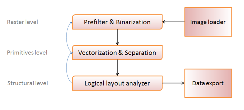
Conventionally, processing methods can be divided into three levels:

Raster level (working with a set of image pixels);
The level of primitives (we identify groups of pixels with certain primitives, - symbols, lines, circles, etc.);
Structural level (we collect groups of primitives into logical units - “table”, “table cell”, “label”, etc.)

I depict the main direction of data transfer with black arrows: load the image, convert it into a convenient form for processing, get primitives, organize primitives into structures, record the result.

Blue arrows represent “feedback” - in some cases, it becomes impossible to recognize an object at a certain level (to collect at least some logically acceptable structure from primitives, or to isolate at least some primitive from a set of points). This indicates either a “bad” source image, or an error in the previous step, and to avoid such errors, we try to process the object again, possibly with different parameters, at the previous structural level.

At this stage, we will not go into details, but these systems of optical recognition of structural information differ significantly from “general recognition” - we have the opportunity to correct some errors thanks to an understanding of the required output structure. This circumstance somewhat changes the approach to the construction of private recognition methods, allowing you to create adaptive algorithms that depend on some tolerances that are modified during the processing and have quality metrics that can be calculated at the structural processing stage.
')

Raster level: image loading

Since we used the wonderful OpenCV library , this step is as simple as possible. OpenCV can load many popular raster formats: PNG, JPG, BMP, DIB, TIFF, PBM, RAS, EXR, and in fact with one line:

cv::Mat mat = cv::imread(fname, CV_LOAD_IMAGE_GRAYSCALE);

The selected parameter CV_LOAD_IMAGE_GRAYSCALE allows you to upload a picture in the form of a matrix of pixel intensities (conversion to grayscale will occur automatically). In a number of tasks it is necessary to use color information, but in ours it is not necessary, which allows you to significantly save memory allocation. From the dirty tricks, except that the download is “transparent” PNG, the transparent background will be treated as black, which can easily be done with the CV_LOAD_IMAGE_UNCHANGED parameter and manual processing of BGRA color information (yes, OpenCV stores the color data in that order).

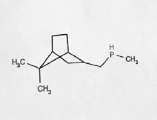
Let at this stage we get something like this:

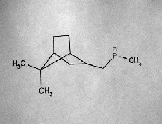
I deliberately chose the picture “worse” to show that optical recognition is associated with numerous difficulties that we will solve further, but it is from “real life” - mobile phone cameras “and they can’t.”

Raster Level: Pre-Filtering

The main task of pre-filtering is to improve the “quality” of the image: remove noise, without loss of detail and restore contrast.

Armed with a graphical editor, you can estimate a lot of tricky schemes, how to improve the quality of the image, but here it is important to understand the boundary between what can be done automatically and what is fiction that applies to exactly one image. Here are examples of more or less automated approaches: sparse masks , median filters , for those who like to google .

I would like to make a comparison of the methods and show why we chose a specific one, but practically it’s difficult. In various images, certain methods have their advantages and disadvantages, “on average” there is no better solution either, so we designed a stack of filters in Imago OCR, each of which can be used in certain cases, and the choice of result will depend on the quality metric.

But I want to talk about one interesting solution: Retinex Poisson Equation

The advantages of the method include:

Fairly high speed;
Parameterized result quality;
The lack of blurring during the work, and as a result, "sensitivity" to the details;
And the main interesting feature is the normalization of local levels of illumination.

The last property is perfectly illustrated by the image from the article, and it is important for recognition because of possible non-uniform illumination of objects when shooting (a piece of paper turned towards the light source so that the light falls unevenly):

Surface description of the algorithm:

Local threshold image filtering ( laplacian threshold ) with a threshold T;
Discrete cosine transformation of the resulting image;
Filtering high-frequency characteristics and solving a special equation for low and medium frequencies (Retinex Equation);
Inverse discrete cosine transform.

The algorithm itself is rather sensitively dependent on the parameter T, but we used its adaptation:

Consider Retinex (T) for T = 1,2,4,8
Perform pixel median filtering between Retinex results.
Normalize the contrast

What will help OpenCV: there is a ready function for calculating the discrete cosine transform:

 void dct(const Mat& src, Mat& dst, int flags=0); // flags = DCT_INVERSE for inverse DCT

And it works no worse in speed than the similar one from libfftw, although I don’t presume to assert this in the general case (tested on Core i5, Core Duo).

For the original image, the above method gives a rather pleasant result:

Now we roughly understand what pre-filtering should do, and we already have one parameter that can change in the feedback mechanism: the index of the filter used .

Here and below : in fact, of course, there are many other parameters (for example, the very “magic” T = 1, 2, 4, 8), but in order “not to bother with the head”, we will not talk about them now. There are many of them, mentions about them will pop up in the section on machine learning, but I’ll omit the specifics in order not to overload the presentation with a number of parameters.

Raster level: binarization

The next step is to get a black and white image, where black will respond to the presence of "paint", and white - to its absence. This is done because a number of algorithms, such as obtaining the contour of an object, do not work constructively with semitones. One of the simplest ways to binarize is threshold filtering (we choose t as the threshold value, all pixels with intensity greater than t are background, less are paint), but because of its low adaptivity , the otsu threshold or adaptive gaussian threshold is often used.

Despite the adaptability of more advanced methods, they still contain threshold values that determine the "amount" of output. In the case of more severe thresholds - some of the elements may be lost, in the case of "soft" - "noise" may come out.

Strong thresholding	Weak thresholding

You can try to guess the thresholds for each image exactly, but we went the other way - using the correlation between the obtained images with different adaptive binarization thresholds:

We consider strong and weak binarization (with given thresholds t1 and t2);
We divide the images into a set of connected pixel-by-pixel areas ( marking of segments );
Remove all the "weak" segments that have a correlation with the corresponding strong, less than the specified (cratio);
Remove all the “weak” segments of low density (the proportions of black / white pixels are less than the given bwratio);
The remaining "weak" segments are the result of binarization.

As a result, in most cases, we obtain an image that is devoid of noise and without loss in detail:

The described solution may look strange in the light of the fact that we wanted to “get rid” of one parameter, and introduced a whole bunch of others, but the basic idea is that the correctness of binarization is now provided if the “real” threshold of binarization falls within the interval , concluded between the t1 and t2 chosen by us (although we cannot increase this interval infinitely, there is also a limit to the difference between t1 and t2).

The idea is quite viable when applied with various methods of threshold filtering, and OpenCV “helped” with the presence of built-in adaptive filtering functions:

 cv::adaptiveThreshold(image, strongBinarized, 255, cv::ADAPTIVE_THRESH_GAUSSIAN_C, CV_THRESH_BINARY, strongBinarizeKernelSize, strongBinarizeTreshold); cv::threshold(image, otsuBinarized, otsuThresholdValue, 255, cv::THRESH_OTSU);

If the final image contains no segments at all, then a filtering error probably occurred and it is worth considering another preliminary filter (“feedback”; “those” blue arrows in the image of the engine structure).

Level of primitives: vectorization

The next step in the recognition process is the conversion of sets of pixels (segments) into primitives. Primitives can be figures - a circle, a set of segments, a rectangle (a specific set of primitives depends on the problem to be solved), or symbols.

So far we don’t know to which class each object belongs, therefore we are trying to vectorize it in various ways. The same set of pixels can be successfully vectorized as a set of segments and as a symbol, for example, “N”, “I”. Or the circle and symbol - “O”. At this stage, we do not need to know reliably which class has an object, but it is necessary to have a certain metric of the object's similarity with its vectorization in a certain class. This is usually solved by a set of recognition functions.

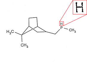
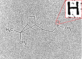
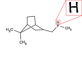
For example for a set of pixels

we will get a set of the following objects (do not think about the specific numbers of the metric, they are given to represent what we want from the recognition process, but by themselves do not make sense yet):

vectorization in the form of the symbol “H” with the metric (distance) value of 0.1 (perhaps it is H) ;
vectorization in the form of the symbol “R” with the value of the metric in 4.93 (unlikely, but it is also possible that R) ;
vectorization in the form of three segments "|", "-", "|" with a metric value of 0.12 (it is quite possible that these are three segments) ;
vectorization as a rectangle with the sizes of the sides x, y with the value of the metric in 45.4 (it does not look like a rectangle at all) ;
vectorization as a circle with the value of the metric + inf (guaranteed is not a circle) ;
...

In order to get a list of vectorizations, it is necessary to implement recognition primitives for each particular class.

Recognition of a set of segments

Usually the raster area is vectorized into a set of segments as follows:

Performing thinning filter ( -> );
Segmentation (decorner) ( );
Approximation of points of each segment;
The result is a set of approximations and a deviation of the approximation from the original.

There is no ready-made thinning filter in OpenCV, but it's not at all difficult to implement. Splitting into segments (decorner), too, but this is completely trivial: we throw out from the area all points that have more than two neighbors. But the approximation of points as a set of segments in OpenCV is present, we used it:

 cv::approxPolyDP(curve, approxCurve, approxEps, closed); // approximation of curve -> approxCurve

An important parameter is the approximation tolerance ( approxEps ), with an increase in which, as a result, we will get a larger number of segments, and with a decrease, a more rough approximation, and, as a result, a larger metric value. How to choose it correctly ?

Firstly, it depends quite strongly on the average line thickness (intuitively - the greater the line thickness, the less detail; the picture drawn with a sharp pencil can be much more detailed than that drawn with a marker), which we used in our implementation:

 approxEps = averageLineThickness * magicLineVectorizationFactor;

Secondly, taking into account the above described approach to the classification of objects, there is an opportunity to try to vectorize segments with different approxEps (with a certain step) and already at the stage of analyzing the logical structure, choose the “more suitable” one.

Circle Recognition

Pretty simple:

Looking for the center of the circle (average over the coordinates of the points) - (x, y);
We are looking for the radius (the average distance of points from the center) - r;
We consider the error: the average distance by points to a circle with center (x, y) and radius r and thickness averageLineThickness;
Consider an additional penalty for breaking a circle: magicCirclePenalty * (% breaks).

After selecting magicCirclePenalty with this code, there were absolutely no problems, as well as with the recognition of rectangles similar to it.

Character Recognition

Significantly more interesting part, because This is a challenge problem - there is not a single algorithm that claims to be “the most optimal” recognition indicators. There are very simple methods based on heuristics , there are more complex ones, for example, using neural networks , but none of them guarantee “good” quality of recognition.

Therefore, it seemed rather natural to decide to use several subsystems of character recognition and selection of an aggregate result: if p1 = the metric value of the fact that algorithm 1 recognizes area A as a symbol s, and p2 = the metric value that algorithm 2 recognizes area A as a character s, total value p = f (p1, p2). We have chosen two algorithms that have conveniently compared values, high speed and sufficient stability:

recognition based on Fourier descriptors;
mask square deviation points.

Character recognition based on Fourier descriptors

Training:

Getting the outer contour of the object;
Converting the coordinates of contour points (x; y) into complex numbers x + iy;
The discrete Fourier transform of a set of these numbers;
Dropping the high-frequency part of the spectrum.

When performing the inverse Fourier transform, we get a set of points describing the original shape with a given degree of approximation (N is the number of coefficients left):

The “recognition” operation is to compute the Fourier descriptors for the recognized area and compare them with the predefined sets responsible for the supported characters. To get a metric value from two sets of descriptors, you need to perform an operation called convolution: d = sum ((d1 [i] -d2 [i]) * w [i], i = 1, N), where d1 and d2 are sets of descriptors Fourier, and w is the weights vector for each coefficient (we received it by machine learning). The value of the convolution is invariant with respect to the scale of the compared characters. In addition, the function is resistant to high-frequency noise (random pixels that do not change the "geometry" of the shape).

OpenCV is quite helpful in implementing this method; There is a ready-made function for obtaining external contours of objects:

 cv::findContours(image, storage, CV_RETR_EXTERNAL);

And there is the calculation function of the discrete Fourier transform:

 cv::dft(src, dst);

It remains only to implement convolution and intermediate type conversions, saving a set of descriptors.

The method is good for handwritten characters (perhaps, probably because others give less qualitative results against it), but it is not suitable for small resolution characters because high-frequency noise, that is, “extra” pixels become large with respect to the entire image and begin to influence those factors that we do not discard. You can try to reduce the number of compared coefficients, but then it becomes more difficult to choose from similar small characters. And so another recognition method was introduced.

Character recognition based on square deviation masks

This is quite an intuitive solution, which, as it turned out, works great for printable characters of any permissions; if we have two black and white images of the same resolution, then we can learn to compare them pixel-by-pixel.

For each point of the image 1 is considered fine: the minimum distance to the point of the image 2 of the same color. Accordingly, a metric is simply a sum of penalties with a normalizing factor. Such a method will be much more stable on low-resolution images with noise — for an image with a side length n, individual pixels up to k percent do not “spoil” the metric by more than k * n in the worst case, and in practical cases by no more than k , because in most cases they are adjacent to the “right” pixels of the image.

The disadvantage of the method, in the description as I described, will be the low speed of work. For each pixel (O (n ² )) we consider the minimum distance to a pixel of the same color of another picture (O (n ² )), which gives O (n ⁴ ).

But this is quite easily treated with a precomputation: we construct two masks, penalty_white (x, y) and penalty_black (x, y), in which the precomputed penalties for pixel (x, y) turn out to be white or black, respectively. Then the process of "recognition" (that is, the calculation of the metric) fits into O (n ² ):

 for (int y = 0; y < img.cols; y++) { for (int x = 0; x < img.rows; x++) { penalty += (image(y,x) == BLACK) ? penalty_black(y,x) : penalty_white(y,x); } }

It remains only to store masks (penalty_white, penalty_black) for each writing of each character and in the process of recognizing them to go through. OpenCV practically does not help us with the implementation of this algorithm, but it is trivial. But, as I have already said, the compared images must be of the same resolution, therefore, in order to bring one to the other, a function may be required:

 cv::resize(temp, temp, cv::Size(size_x, size_y), 0.0, 0.0);

If we go back to the general process of character recognition, then as a result of running both methods, we get a table of metric values:

The recognition value is not one element, but the entire table, from which we know that with the greatest probability is the “C” symbol, but perhaps it is “0” or “6” (or “O”, or “c”, which did not fit on the screen). And if it is a bracket, then it is more likely to open than to close. But for now we don’t even know if this is a symbol at all ...

Primitive Level: Separation

If we lived in the ideal world of superproductive (quantum?) Computers, then most likely this step would not be necessary: we have a set of some objects, for each of which there is a table of “probabilities” defining what it is. We iterate over all the elements in the table for each object, build a logical structure, and choose the most likely (by the sum of the metrics of individual objects) from the valid ones. Delov something, except perhaps the exponential complexity of the algorithm.

But in practice it is usually necessary to determine the type of object by default. That is, to choose some finished interpretation of objects in the image, and then, perhaps slightly change it. Why we could not choose the type of objects in the previous step (vectorization)? We did not have enough statistical information about all objects, and if we interpret a certain set of pixels in isolation from the entire picture, then reliably determine its meaning becomes problematic.

This is one of the most important issues of recognition of structural information. In humans, this is much better than the car, because he simply does not know how to see the pixels separately. And one of the initial stages of disappointment in building an OCR system is an attempt to algorithmize a sort of “step-by-step” human approach, while at the same time obtaining unsatisfactory results. It seems that just now, it is worthwhile to slightly improve the recognition algorithms of primitives so that they “do not make mistakes” and we will get better results, but there are always a few pictures that “break” any logic.

And so, we ask the person what it is -

Of course, this is just a curved line. But if it is necessary to rank it either as symbols or as a set of straight line segments, what is it? Then it is most likely either the letter “l” or two straight lines at an angle (just the corner is drawn rounded). But how to choose the right interpretation? The machine could have solved the approximate problem at the previous step, and solved it correctly with a probability of 1/2. But 1/2 is a complete breakdown for the structural information recognition system, we just spoil the structure, it does not pass validation, it is necessary to correct "errors" that, by a happy probability, may not coincide with the true problem. .

, :

, - (, ). , , , « » — .

:

, , «» , , . , , , — . , «Cl» () , , - «l».

. .

:

«» ( ), C, .

, .

:

;
, ;
;
, ;
, hu moments ( OpenCV ).

, — , , — " ".

, : ( __-1 __+2, 3*__ 0.5* ), . , .

. — . , , - ( ). «» ( — , «l» , «l». , ).

:

;
, ;
: , .

« » — .

, , .

. , .

, Imago OCR , , ( ), . , . , . , .

, . , — , «» «», :

, «» , :

— . , , , , .

:

— (, ). , , , — ( , — ).

, . , «» ( ), «». , , — «» .

, «» . , — .
« » :

( baseline_y), , — . baseline_y :

( );
y , .

, ( )? ; , , , « ». baseline_y , — .

, . :

% , ;
.

: 30% — . 29? duck test. - , — . , - .

? , . . ( , ?). . , :

k% , f(k) ;
n% , , a..z g(n) .

, — , . «» .

— . — : — , , — . .

: {c1, c2}
c1 — «Y» 0.1 «X» 0.4;
c2 — «c» 0.3 «e» 0.8
, — Yc . Yc . . — .
4 , " Xe ", 1.2.

, . , «Yc» , . , (1.2) (0.4), (0.8). , , . ?

, , ? , , ?

— , . , , .

, — , . , . .

, , , , , , ; ( ) . , , — .

Instead of conclusion

« » OCR , . , , , , . .

, , open-source Imago OCR , google .

Source: https://habr.com/ru/post/172651/

All Articles