Recognizing gender in images and videos
This article presents a gender recognition algorithm with an accuracy of 93.1% [1] . The article does not require any prior knowledge in image processing or machine learning. After reading the article, the reader will be able to execute the considered algorithm on his own.
Looking at the person, we usually accurately determine the sex. Sometimes we make mistakes, but often in such cases it is really difficult to do.
Often we use some context. For example, for the author of an article, the color of clothes is sometimes the most significant sign when trying to identify the sex of a child up to 1-2 years.
')
Let us turn to the problem of determining the sex of the face. We want to refer each face image to either a class of men or a class of women. We need a mechanism that will decide which class the photo belongs to. In such a formulation, the problem looks like a typical machine learning task: there is a set of labeled examples of two classes: M and J. “Marked” means that each photo is mapped to the floor of the person depicted on it. So we need some classifier.
However, on the basis of what the floor classifier will decide which class to include the image in? Looking for some characteristics. Each image is a matrix of a certain size.
whose elements encode the brightness of each pixel. Obviously, you can use image pixels directly. This approach often gives good results, but it is unstable to changes in lighting and the presence of noise in the image.
Another approach is to use some pixel ratios. Developed a huge number of such relationships or characteristics (features). The study of the applicability of a particular type of characteristic is a key stage in many computer vision tasks.
To solve the problem of gender recognition, the authors of the article Boosting Sex Identification Performance [1] propose to use the set of simple features described below.
For simplicity, we number all pixels in the image: - means the brightness of a pixel with a serial number
. Consider the following set of characteristics ( 
):
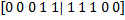
In other words, we compose all possible pairs of pixels in the image, calculate their difference and apply the rules described above. Each comparison gives a binary characteristic. For example, for
 we have:
Thus, we have a vector of characteristics . To these five characteristics are added their inverse characteristics -
  . Combining these vectors, we get the following set of binary characteristics for
  and
and  :
:  . The reader may have a logical question: why should the data that is obtained by negating the data that already exist in it be entered into the training sample? Why do we need this redundancy? Good question! The answer to it will become clear later when creating a classifier.
Thus, for each pair of pixels we have 10 characteristics; for the image pixels we get
  characteristics. Once again, we note that the characteristics in our context are just pixel differences with the rules described above.
Obviously, not all characteristics should be used for gender recognition. Moreover, processing such a large number of numbers may be inefficient. Surely, among this set of characteristics, there is a small part of those that encode gender differences better than others. So how to choose such characteristics?
This problem is effectively solved using the AdaBoost algorithm [2] [3] , the goal of which is to select a small set of valuable characteristics from a very large initial array.
Let's start with the preparation of data. For training and testing, we will use the FERET database [4] [5] . It contains various photos of 994 people (591 men, 403 women), and, for each person, there are several photos taken in different poses.
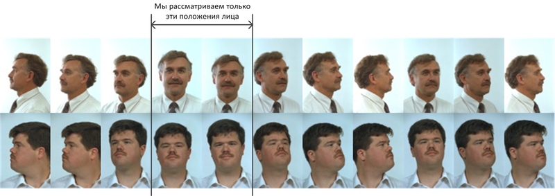
On each photo you need to find the eyes, cut out the area of interest to us and reduce it to size.

Fortunately, the creators of FERET marked the main points on the face manually, and the eyes among them. However, in a real recognition system, the eyes are arranged with a special algorithm, which is usually less accurate than manual placement. Therefore, for cutting out areas of interest at the stage of learning to recognize sex, it is recommended to use the same eye placement algorithm that will be in the recognition system. In this case, the classifier “learns” to take into account the alignment error of the eyes by the algorithm.
As a result of pre-processing, we have two sets of pictures:
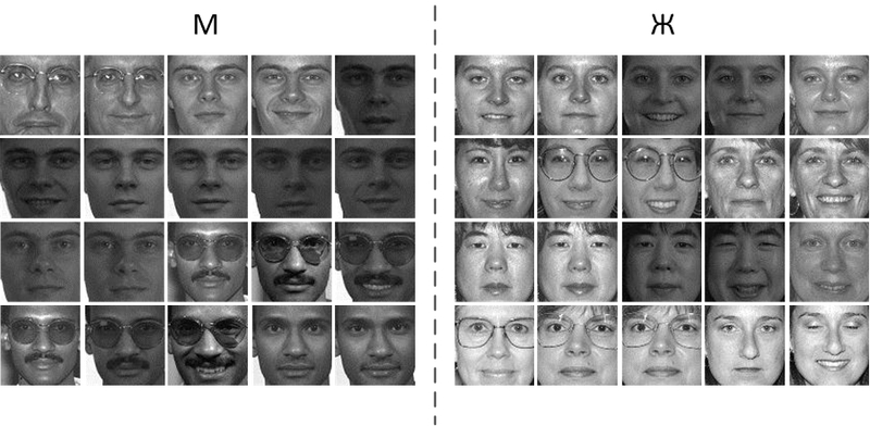
Note that for clarity, each person in the figure above has dimensions pixels, in fact, in the considered approach images are used pixels The training set will be used to train the classifier, as the name suggests. The test sample is “unknown” to the classifier, so it can be used to objectively measure the accuracy indicators.
Therefore, it is necessary
The figure below shows the matrix of input and output data. Such a pair must be composed for both the training set and the test sample.
Now we will try to understand the learning algorithm “in words”. A little below is the formal scheme of the AdaBoost algorithm.
Recall that our task is to select such characteristics that can best divide the classes M and J. Suppose that we have already analyzed such characteristics in order, and proceed to the analysis
:

Meanings characteristics for the first three teaching examples  the value of the label vector for these examples
  . If you accept the values characteristics as a gender prediction, the error vector in this case will be
  . If we consider the characteristic
  then
then  . Thus, choosing between characteristics
  and , should prefer the characteristic , because
 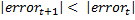 . After going through all the characteristics, we will find T best, which we will use for classification.
And now the formal learning procedure.
Teaching examples: where
where  - image,
  in the case of the female,
  in the case of masculine.
Initializing the weights vector :
:
Where and
and  the number of examples of female and male, respectively.
For (where T is the number of characteristics we want to choose)
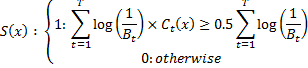
The resulting classifier is represented by the formula:
Let's try to estimate the range of values that can take . We have already noted that
  takes values on a segment
  . Now suppose that
  for some classifier
  . Obviously, in this case
  . However, will such a classifier be chosen by the algorithm described above? Obviously, it will not, because there will always be such a classifier in the training sample
  obtained by using the negation operation
  , for which
  and
and  . It is easy to see that if the example was classified correctly, then its weight is reduced by multiplying by
  , and thus, examples that are classified incorrectly (complex examples) gain more weight.
Now back to the question of redundancy, which we asked earlier. Presence in the sample of classifiers obtained by negation , limits on the segment  and allows weights of complex examples to grow.
Given the size of the input matrices, the choice of the first 1000 characteristics of the standard AdaBoost algorithm takes about 10 hours (Intel Core i7). Standard, then, running on all the characteristics. There are versions of the algorithm that work with random characteristics from the entire set, but their description is beyond the scope of this article. A training time of 10 hours is an acceptable result for this task, as this is a one-time operation.
Note that the algorithm results in pairs of pixel indices to be compared, one of the five comparison rules and the value for each pair. In fact, for the analysis of the photograph, it is only necessary to calculate the differences, apply the selected rule and find a solution using the formula for  . Therefore, this algorithm is absolutely not demanding of resources and does not slow down the recognition system in which it is used.
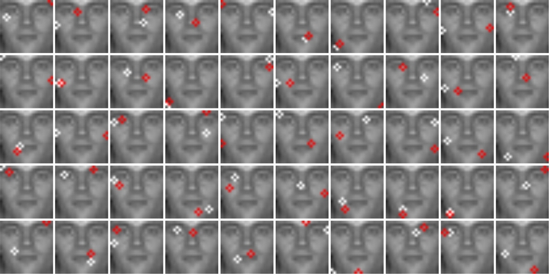
Now the fun part! What characteristics chose AdaBoost ?! Below are the first 50 features that AdaBoost has chosen. Red and white pixels are and  . When analyzing pixels around the edges of an image, you must remember that the faces of many people do not fit into the frame. Therefore, edge pixels can, in some way, encode the size of a face.
Consider the dependence of the classification accuracy on the number of used characteristics.

Note that the graph was obtained using data from the FERET database, which AdaBoost “did not see” at the training stage. Maximum accuracy of 93.1% is achieved using 911 characteristics. The authors of this approach report an accuracy of 94.3%, which is very close to the obtained indicator. The difference of 1.2% may occur due to different splitting into training and test samples. Also in this article, an own algorithm was used to search for eyes, the accuracy of which differs from the accuracy of the human arrangement of eyes in the FERET database.
However, what if the classifier learned to recognize only the base on which it was trained ?! A similar effect occurs when a student, preparing for an exam, simply learns formulas, tasks, examples, without understanding the essence. Such a student is able to solve only those tasks that he has already seen, and is not able to extend his knowledge to new problems. This effect in machine learning is called overfitting (retraining) and is a serious problem in recognition. The opposite effect is called generalization.
To test the ability to generalize, we will use another database of individuals - Bosphorus Database [6] [7] . It consists of photos of 105 people. The base contains up to 35 different facial expressions for each person.
The graph below is similar to the graph presented a little higher, with the only difference that is obtained using the Bosphorus Database (that is, the possibility of becoming acquainted with the test sample is excluded).

The test sample includes 1300 photographs (727 M and 573 F). Maximum accuracy of 91% is achieved with 954 specifications. Note that the mark of 90% is achieved already with 100 characteristics.
These two graphics, as well as the videos that are present in the article, demonstrate the high accuracy of this approach on the data that he "did not see" at the training stage. That is why it is considered the state-of-the-art algorithm for gender recognition.
The following video shows the work of the algorithm on the fragments of TV shows. To achieve this accuracy, “smoothing” of results over time is used: each face is observed for 19 frames, each of which determines the gender. The result is the gender that has been encountered the most times in the last 19 frames.
Introduction
Looking at the person, we usually accurately determine the sex. Sometimes we make mistakes, but often in such cases it is really difficult to do.
Often we use some context. For example, for the author of an article, the color of clothes is sometimes the most significant sign when trying to identify the sex of a child up to 1-2 years.
')
Let us turn to the problem of determining the sex of the face. We want to refer each face image to either a class of men or a class of women. We need a mechanism that will decide which class the photo belongs to. In such a formulation, the problem looks like a typical machine learning task: there is a set of labeled examples of two classes: M and J. “Marked” means that each photo is mapped to the floor of the person depicted on it. So we need some classifier.
However, on the basis of what the floor classifier will decide which class to include the image in? Looking for some characteristics. Each image is a matrix of a certain size.
Another approach is to use some pixel ratios. Developed a huge number of such relationships or characteristics (features). The study of the applicability of a particular type of characteristic is a key stage in many computer vision tasks.
Specifications
To solve the problem of gender recognition, the authors of the article Boosting Sex Identification Performance [1] propose to use the set of simple features described below.
For simplicity, we number all pixels in the image:
- means the brightness of a pixel with a serial number 


In other words, we compose all possible pairs of pixels in the image, calculate their difference and apply the rules described above. Each comparison gives a binary characteristic. For example, for
we have: - false (0)
 - false (0)
 - false (0)
 - true (1)
 - true (1)
Thus, we have a vector of characteristics
. To these five characteristics are added their inverse characteristics - . Combining these vectors, we get the following set of binary characteristics for and : . The reader may have a logical question: why should the data that is obtained by negating the data that already exist in it be entered into the training sample? Why do we need this redundancy? Good question! The answer to it will become clear later when creating a classifier.Thus, for each pair of pixels we have 10 characteristics; for the image
pixels we get characteristics. Once again, we note that the characteristics in our context are just pixel differences with the rules described above.Obviously, not all characteristics should be used for gender recognition. Moreover, processing such a large number of numbers may be inefficient. Surely, among this set of characteristics, there is a small part of those that encode gender differences better than others. So how to choose such characteristics?
This problem is effectively solved using the AdaBoost algorithm [2] [3] , the goal of which is to select a small set of valuable characteristics from a very large initial array.
Data preparation and classifier training
Let's start with the preparation of data. For training and testing, we will use the FERET database [4] [5] . It contains various photos of 994 people (591 men, 403 women), and, for each person, there are several photos taken in different poses.
On each photo you need to find the eyes, cut out the area of interest to us and reduce it to size.
Fortunately, the creators of FERET marked the main points on the face manually, and the eyes among them. However, in a real recognition system, the eyes are arranged with a special algorithm, which is usually less accurate than manual placement. Therefore, for cutting out areas of interest at the stage of learning to recognize sex, it is recommended to use the same eye placement algorithm that will be in the recognition system. In this case, the classifier “learns” to take into account the alignment error of the eyes by the algorithm.
As a result of pre-processing, we have two sets of pictures:
Note that for clarity, each person in the figure above has dimensions
pixels, in fact, in the considered approach images are used pixels The training set will be used to train the classifier, as the name suggests. The test sample is “unknown” to the classifier, so it can be used to objectively measure the accuracy indicators.Therefore, it is necessary
- For each photo, compile a vector of binary characteristics (weak classifiers) containing
 items
items - “Pack” such vectors of all photos in two matrices:
 and
and 
- Create the corresponding output vectors in which
 the element takes the value 1 if
  photo belongs to a man, otherwise 0
The figure below shows the matrix of input and output data. Such a pair must be composed for both the training set and the test sample.
Now we will try to understand the learning algorithm “in words”. A little below is the formal scheme of the AdaBoost algorithm.
Recall that our task is to select such characteristics that can best divide the classes M and J. Suppose that we have already analyzed
such characteristics in order, and proceed to the analysis Meanings
characteristics for the first three teaching examples the value of the label vector for these examples . If you accept the values characteristics as a gender prediction, the error vector in this case will be . If we consider the characteristic then . Thus, choosing between characteristics and , should prefer the characteristic , because . After going through all the characteristics, we will find T best, which we will use for classification.And now the formal learning procedure.
Teaching examples:
where - image, in the case of the female, in the case of masculine.Initializing the weights vector
: if the i-i picture is female
 if i-i picture is male
Where
and the number of examples of female and male, respectively.For
(where T is the number of characteristics we want to choose)- Normalization of scales, so that
 .
. - For each weak classifier,
 , we consider the classification error taking into account weights:
  . For each example, the error takes on the value either 0 if the classification is correct or
  in case of wrong. Because then
  .
. - Choosing a classifier
 with the least error
  and see how it classifies the data.
 - Update weights.
If the example is classified incorrectly (i.e. ),
), .
.
Otherwise ,
,
Where .
.
The resulting classifier is represented by the formula:
Let's try to estimate the range of values that can take
. We have already noted that takes values on a segment . Now suppose that for some classifier . Obviously, in this case . However, will such a classifier be chosen by the algorithm described above? Obviously, it will not, because there will always be such a classifier in the training sample obtained by using the negation operation , for which and . It is easy to see that if the example was classified correctly, then its weight is reduced by multiplying by , and thus, examples that are classified incorrectly (complex examples) gain more weight.Now back to the question of redundancy, which we asked earlier. Presence in the sample of classifiers obtained by negation
, limits on the segment and allows weights of complex examples to grow.Given the size of the input matrices, the choice of the first 1000 characteristics of the standard AdaBoost algorithm takes about 10 hours (Intel Core i7). Standard, then, running on all the characteristics. There are versions of the algorithm that work with random characteristics from the entire set, but their description is beyond the scope of this article. A training time of 10 hours is an acceptable result for this task, as this is a one-time operation.
Note that the algorithm results in pairs of pixel indices to be compared, one of the five comparison rules and the value
for each pair. In fact, for the analysis of the photograph, it is only necessary to calculate the differences, apply the selected rule and find a solution using the formula for . Therefore, this algorithm is absolutely not demanding of resources and does not slow down the recognition system in which it is used.results
Now the fun part! What characteristics chose AdaBoost ?! Below are the first 50 features that AdaBoost has chosen. Red and white pixels are
and . When analyzing pixels around the edges of an image, you must remember that the faces of many people do not fit into the frame. Therefore, edge pixels can, in some way, encode the size of a face.Consider the dependence of the classification accuracy on the number of used characteristics.
Note that the graph was obtained using data from the FERET database, which AdaBoost “did not see” at the training stage. Maximum accuracy of 93.1% is achieved using 911 characteristics. The authors of this approach report an accuracy of 94.3%, which is very close to the obtained indicator. The difference of 1.2% may occur due to different splitting into training and test samples. Also in this article, an own algorithm was used to search for eyes, the accuracy of which differs from the accuracy of the human arrangement of eyes in the FERET database.
However, what if the classifier learned to recognize only the base on which it was trained ?! A similar effect occurs when a student, preparing for an exam, simply learns formulas, tasks, examples, without understanding the essence. Such a student is able to solve only those tasks that he has already seen, and is not able to extend his knowledge to new problems. This effect in machine learning is called overfitting (retraining) and is a serious problem in recognition. The opposite effect is called generalization.
To test the ability to generalize, we will use another database of individuals - Bosphorus Database [6] [7] . It consists of photos of 105 people. The base contains up to 35 different facial expressions for each person.
The graph below is similar to the graph presented a little higher, with the only difference that is obtained using the Bosphorus Database (that is, the possibility of becoming acquainted with the test sample is excluded).
The test sample includes 1300 photographs (727 M and 573 F). Maximum accuracy of 91% is achieved with 954 specifications. Note that the mark of 90% is achieved already with 100 characteristics.
These two graphics, as well as the videos that are present in the article, demonstrate the high accuracy of this approach on the data that he "did not see" at the training stage. That is why it is considered the state-of-the-art algorithm for gender recognition.
The following video shows the work of the algorithm on the fragments of TV shows. To achieve this accuracy, “smoothing” of results over time is used: each face is observed for 19 frames, each of which determines the gender. The result is the gender that has been encountered the most times in the last 19 frames.
Links
- S. Baluja, and H. Rowley, Boosting Sex Identification Performance , International Journal of Computer Vision, v. 71 i. 1, January 2007
- Y. Freund and R. Shapire, “A decision-theoretic generalization of on-line learning and an application to boosting” , Journal of Computer and System Sciences, 1996 pp. 119-139
- Y. Freund and R. Shapire, “A Short Introduction to Boosting” , Journal of Japanese Society for Artificial Intelligence, 14 (5): 771-780, September, 1999
- PJ Phillips, H. Moon, SA Rizvi and PJ Rauss, "The FERET evaluation methodology for face recognition algorithms," IEEE Trans. Pattern Analysis and Machine Intelligence, Vol. 22, pp. 1090-1104, 2000
- http://www.itl.nist.gov/iad/humanid/feret/feret_master.html
- Bosphorus Database
- A. Savran, B. Sankur, MT Bilge, “Comparative Evaluation of the Universe”, Pattern Recognition, Vol. 45, Issue 2, p767-782, 2012.
Source: https://habr.com/ru/post/172463/
All Articles