Performance test: amazing and simple
It so happened that for the last six months I have been actively engaged in performance tests and it seems to me that in this area of IT there is an absolute lack of understanding of what is happening. Nowadays, when the growth of computing power has decreased (vertical scalability), and the volume of tasks is growing at the same speed, the problem of performance is becoming more acute. But before you rush into the fight against performance, you need to get a quantitative description.
Summary of the article:
Once, traveling in a train, I wanted to calculate the distance between the power poles. Armed with the usual clock and estimating the average train speed of 80-100km / h (25 m / s), I marked the time between 2 pillars. Oddly enough, this naive method gave a very depressing result, up to 1.5-2 times the difference. Naturally the method was easy to fix, which I did, it was enough to detect 1 minute and count the number of pillars. And it does not matter that the instantaneous speed over a minute can vary and it doesn’t even matter that we count the last pillar or minute in the middle, because measurements are quite enough for the desired result.
The meaning of the test is to get convincing for yourself and for other measurements.
')
This story reminds me of what happens with software engineering performance testing. A rather frequent phenomenon is the launch of 1-2 tests, the construction of graphs and the drawing of conclusions about the scalability of the system. Even if it is possible to use MNCs or find out a standard error, this is not done because of “uselessness.” The situation is especially interesting when, after these 2 measurements, people discuss how fast the system is, how it scales and compare it with other systems for personal sensations.
Of course, it is not difficult to estimate how fast the team is executed. On the other hand, faster does not mean better. Software systems have over 10 different parameters, from hardware on which they operate to input, which the user enters at different points in time. And often 2 equivalent algorithms can produce completely different scalability parameters in different conditions, which makes the choice not at all obvious.
On the other hand, measurement results always remain a source of speculation and distrust.
- Yesterday we measured was X, and today 1.1 * X. Someone changed something? - 10% - this is normal, we now have more records in the database.
- During the test, the antivirus, skype, screensaver animation was disabled?
“No-no, for normal tests we need to purchase a cluster of servers, set up microsecond time synchronization between them ... remove the OS, run in protected mode ...
- How many users do we support? We have 5000 registered users, suddenly 20% of them will log in, it is necessary to run tests with 1000 parallel agents.
First, we have to admit that we already have the iron that we have, and we need to get maximum results on it. Another question is how we can explain the behavior on other machines (production / quality testing). Those who advocate for the experiments of "clean room" simply do not trust you, since you do not give enough explanations or data, "clean room" is an illusion.
Secondly, the most important advantage in testing programs is the low cost of tests. If physicists could conduct 100 tests of a simplified situation instead of 5 full-fledged ones, they would definitely choose 100 (and for checking the results 5 full-fledged :)). In no case, you can not lose the cheapness of tests, run them at home, at a colleague, on the server, in the morning and at lunch. Do not be tempted by the “real” hourly tests with thousands of users, it’s more important to understand how the system behaves than to know a couple of absolute numbers.
Third, store the results. The value of the tests are the measurements themselves, not the conclusions. The findings are far more often wrong than the measurements themselves.
So, our task is to conduct a sufficient number of tests in order to predict the behavior of the system in a given situation.
Immediately make a reservation that we consider the system as a "black box". Since systems can work under virtual machines, with or without a database, it does not make sense to dismember the system and take measurements in the middle (this usually leads to unrecorded important points). But if there is an opportunity to test the system, in different configurations, this should definitely be done.
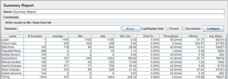
For testing, even a simple test, it is better to have an independent system like JMeter, which can calculate the results, average. Of course, setting up the system takes time, but I want to get the result much faster and we write something like that.
Running once we get the number X. Run again we get 1.5 * X, 2 * X, 0.7 * X. In fact, it is possible and necessary to stop here if we take a temporary measurement and we do not need to insert this number into the report. If we want to share this number with someone, it is important for us that it converges with other dimensions and does not arouse suspicion.
The first “logical” step seems to be to put the numbers X and average them, but, in fact, averaging the averages is nothing more than increasing the count for one test. Oddly enough, increasing the count can lead to even more unstable results, especially if you run the test and do something at the same time.
The problem is that the average is not a stable characteristic, one piled test that was performed 10 times longer would be enough for your results not to coincide with others. As it is not paradoxical for simple performance tests, it is desirable to take the minimum execution time . Naturally, the operation () should be measured in this context, usually 100 ms - 500 ms for the system is more than enough. Of course, the minimum time will not be 1 to 1 coincide with the observed effect or with the real one, but this number will be comparable with other measurements.
Quantiles 10%, 50% (median), 90% are more stable than average, and much more informative. We can find out with what probability the request will execute time 0.5 * X or 0.7 * X. There is another problem with them, it is much more difficult to count quantiles on the knee than to take min, max.
JMeter provides a measurement of the median and 90% in the Aggregate Report out of the box, which naturally should be used.
As a result of measurements, we get a certain number (median, minimum or other), but what can we say about our system (function) by one number? Imagine you are automating the process of obtaining this number and every day you will check it when you need to sound the alarm and look for the guilty? For example, here is a typical schedule of the same test every day.
If we want to write a performance report, with one number it will look empty. Therefore, we will definitely test for different parameters. Tests for different parameters will give us a beautiful graph and an idea of the scalability of the system.
Consider a system with one numeric parameter. First of all, you need to select the parameter values. It does not make sense to choose numbers from different ranges, like [1, 100, 10000], you simply carry out 3 completely different incoherent tests and it will be impossible to find dependencies on such numbers. Imagine you want to build a graph, which numbers would you choose? Something similar to [X * 1, X * 2, X * 3, X * 4, X * 5,].
So, choose 5-10 (7 best) control points, for each point we make 3-7 measurements, take the minimum number for each point and build a graph.
As you can see, the points are located exactly around the imaginary straight line. Now we come to the most interesting part of the measurements, we can determine the complexity of the algorithm based on the measurements. Determining the complexity of an algorithm based on tests is much easier for complex programs than analyzing the text of source programs. With the help of the test, you can even find special points when the difficulty changes, for example, the launch of Full GC.
Determining the complexity of the program on the test results is a direct task of the Regression analysis . Obviously, there is no general way to find a function only by a point; therefore, for the beginning, an assumption is made about some dependence, and then it is checked. In our case, and in most others, we assume that the function is a linear relationship.
To search for linear dependence coefficients, there is a simple and optimal OLS method. The advantage of this method is that the formulas can be programmed in 10 lines and they are absolutely clear.
Let's present our calculations in the table.
In the highlighted line we see the linear coefficient of our model, it is equal to 95.54, the free coefficient is 2688. Now we can do a simple but not obvious focus, we can attach importance to these numbers. 95.54 is measured in milliseconds (as are our measurements), 95.54 is the time we spend on each component, and 2688 ms the time we spend on the system itself does not depend on the number of components. This method allowed us to allocate accurately enough the time of the external system, in this case the database, although it is ten times longer than the time of the 1st component. If we used the Time_with_N_component / N formula, we would have to measure for N> 1000 in order for the error to be less than 10%.
The linear coefficient of the model is the most important number of our measurements and oddly enough it is the most stable number of our measurements. The linear coefficient also makes it possible to adequately measure and interpret operations that occur in nanoseconds, and by separating the overhead of the system itself.
The graph shows the results of independent test launches at different times, which confirms the greater stability of the linear coefficient than individual tests.

Using the graph, we can visually see that our measurements really satisfy the linear model, but this method is far from accurate and we cannot automate it. In this case, the Pearson coefficient can help us. This method does show deviations from a straight line, but for 5-10 measurements it is clearly not enough. Below is an example of a clearly non-linear relationship, but the Pearson coefficient is quite high.
Returning to our table, knowing the ovehead of the system (free coefficient), we can calculate the linear coefficient for each measurement, which is done in the table. As we can see the numbers (100, 101, 93, 96, 102, 81, 94, 100, 93, 98) are rather randomly distributed around 95, which gives us weighty reasons to believe that the dependence is linear. Following the letter of mathematics, in fact, the deviations from the average value should satisfy the normal distribution, and to check the normal distribution, it suffices to check the Kolmogorov-Smirnov criterion, but we leave this for the sophisticated testers.
Oddly enough, not all dependencies are linear. The first thing that comes to mind is a quadratic dependence. In fact, quadratic dependency is very dangerous, it kills performance first slowly and then very quickly. Even if you have everything done for a fraction of a second for 1000 elements, then for 10,000 it will already be tens of seconds (multiplied by 100). Another example is sorting, which cannot be solved in linear time. Calculate how applicable the linear analysis method is for algorithms with complexity O (n * log n)
That is, for n> = 1000, the deviation will be within 10%, which is significant, but in some cases it can be applied, especially if the coefficient at log is large enough.
Consider an example of nonlinear dependence.
The first thing to note is negative overhead, for obvious reasons the system cannot have a negative time spent on preparation. The second, looking at the column of coefficients, you can notice a pattern, the linear coefficient falls, and then grows. This is reminiscent of a parabola chart.
Naturally, most systems do not consist of one parameter. For example, a program for reading from a table already consists of 2 parameters, columns and lines. Using parameterized tests, we can calculate what the cost of reading a row of 100 columns (let it be 100ms) and what are the costs of reading a column for 100 rows (let it be 150ms). 100 * 100ms! = 100 * 150ms and this is not a paradox, we just do not take into account that in the speed of reading lines there is already an overhead reading of 100 columns. That is, 100ms / 100 columns = 1ms - this is not the speed of reading a single cell! In fact, 2 measurements will not be enough to calculate the speed of reading a single cell. The general formula is as follows: where A is the cost per cell, B is one line, C is per column:
Let's make a system of equations, taking into account the available values and one more necessary measurement:
From here, we get A = 0.9 ms, B = 10 ms, C = 50 ms.
Of course, having a formula for the similarity of the LMIC for this case, all calculations would be simplified and automated. In general, the general LMIC does not apply to us, because a function that is linear in each of the arguments is not a multidimensional linear function (hyperplane in N-1 space). It is possible to use the gradient method of finding the coefficients, but this will not be an analytical method.
One of the favorite activities with performance tests is extrapolation. Especially people like to extrapolate to an area for which they cannot get values. For example, having 2 cores or 1 core in the system, I would like to extrapolate how the system behaved with 10 cores. And of course, the first wrong assumption is that the dependence is linear. For a normal definition of a linear relationship, it is necessary from 5 points, which of course is impossible to obtain on 2 cores.
One of the closest approximations is the law of Amdal .
It is based on the calculation of the percentage of the parallelized code α (outside the synchronization block) and the synchronized code (1 - α). If one process takes time T on one core, then for multiple running tasks N time will be T '= T * α + (1-α) * N * T. On average, of course, N / 2, but Amdahl admits N. Parallel acceleration, respectively, S = N * T / T '= N / (α + (1-α) * N) = 1 / (α / N + (1 - α )).
Of course, the above graph is not so dramatic in reality (there is a logarithmic scale in X). However, a significant drawback of synchronization blocks is the asymptote. Relatively speaking, it is not possible by increasing the power to overcome the acceleration limit lim S = 1 / (1 - α). And this limit is quite hard, that is, for 10% of synchronized code, the limit is 10, for 5% (which is very good) the limit is 20.
The function has a limit, but it is constantly growing, and from this arises, at first glance, a strange task: to evaluate which hardware is optimal for our algorithm. In reality, it is quite difficult to increase the percentage of paralized. Let us return to the formula T '= T * α + (1-α) * N * T, optimal from the point of view of efficiency: if the kernel is idle, as much time as it will work. That is, T * α = (1-α) * N * T, hence we get N =
α / (1-α). For 10% - 9 cores, for 5% - 19 cores.
The model of acceleration of calculations is theoretically possible, but not always real. Consider a client-server situation where N clients are constantly running some task on the server, one by one, and we do not experience any costs of synchronizing the results, since the clients are not completely dependent! Keeping statistics for example introduces a synchronization element. Having a M-core machine, we expect the average query time T when N <M is the same, and when N> M the query time increases in proportion to the number of cores and users. Calculate throughput as the number of requests processed per second and get the following "ideal" schedule.
Naturally perfect graphics are achievable if we have 0% synchronized blocks (critical sections). Below are the actual measurements of one algorithm with different parameter values.
We can calculate the linear coefficient and build a graph. Also having a machine with 8 cores, it is possible to conduct a series of experiments for 2, 4, 8 cores. From the test results, you can see that a system with 4 cores and 4 users behaves just like a system with 8 cores and 4 users. Of course, this was expected, and gives us the opportunity to carry out only one series of tests for the machine with the maximum number of cores.
The measurement plots are close in value to the Amdal law, but still significantly different. Having measurements for 1, 2, 4, 8 cores, you can calculate the amount of non-parallelized code using the formula
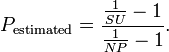
Where NP is the number of cores, SU = Through NP core / Throughput 1 core. According to Amdal's law, this number should be constant, but in all dimensions this number falls, although not significantly (91% - 85%).
The throughput per core chart is not always a continuous line. For example, when there is a shortage of memory or when GC is running, deviations in throughput can be very significant.
When measuring the load on multi-user systems, we introduced the definition of Throughput = NumberOfConcurrentUsers / AverageTimeResponse . To interpret the results. Throughput is the system capacity, how many users the system can serve at a time, and this definition is closely related to queuing theory . The difficulty of measuring throughput is that the value depends on the input stream. For example, in queuing systems, it is assumed that the waiting time for a response does not depend on how many applications are in the queue. In a simple software implementation, without a queue of requests, the time between all threads will be divided and, accordingly, the system will degrade. It is important to note that JMeter does not need to trust throughput measurements, it was noticed that Jmeter averages throughput between all test steps, which is not correct.
Consider the following case: with a load with 1 user, the system issues Throughput = 10, with 2 - Throughput = 5. This situation is quite possible, since the typical Throughput / User graph is a function that has one local (and global maximum).
Therefore, with an incoming stream of 1 user every 125ms, the system will process 8 users per second (input throughput).
With an incoming stream of 2 users every 125ms, the system will begin to collapse, since 8 (input throughput)> 5 (possible throughput).
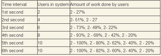
Consider an example of a collapsing system in more detail. After conducting the Throughput / Users test, we have the following results.
Users - the number of simultaneous users in the system; Progress per user - what amount of work as a percentage the user performs in one second. Mentally simulating the situation that 10 users come every second and begin to perform the same operation, the question is whether the system will be able to serve this stream.
In 1 second, 10 users on average will perform only 20% of their work, assuming that on average they perform all in 5. In the 2nd second there will already be 20 users in the system and they will share resources between 20 threads, which will further reduce percentage of work performed. We will continue the row until the moment when the first 10 users finish the work (theoretically they should finish it as the 1/2 / 1/3 + 1/4 row ... divergent).

It is quite obvious that the system will collapse, because after 80 seconds there will be 800 users in the system, and at this point only the first 10 users can finish.
This test shows that for any distribution of the incoming stream, if the incoming throughput (mathematical expectation) is greater than the maximum
measured throughput for the system, the system will begin to degrade and will fall at constant load. But the opposite is not true, in the 1st example, the maximum measured throughput (= 10)> incoming (8), but the system also cannot cope.
An interesting case is a workable system. Taking our measurements as a basis, we will test that every 1 second there are 2 new users. Since the minimum response time exceeds one second, at first the number of users will accumulate.
As we can see, the system will enter the stationary mode exactly at that point, the graphics when the measured throughput coincides with the input throughput. The average number of users in the system will be 10.
From this we can conclude that the Throughput / Users graph on the one hand represents the number of users processed per second (throughput) and the number of users in the system (users). The fall of the graph to the right of this point characterizes only the stability of the system in stressful situations and dependence on the nature of the incoming distribution. In any case, conducting tests Throughput / Users, it is not at all superfluous to conduct a behavioral test with approximate characteristics.
When conducting performance tests, there are almost always measurements that take much longer than expected. If the testing time is long enough, then you can observe the following picture. How to choose one number from all these dimensions?
The simplest statistic is the average, but for the above reasons it is not quite stable, especially for a small number of measurements. To determine the quantile convenient to use the graph of the distribution function. Thanks to the wonderful JMeter plugin , we have this opportunity. After the first 10-15 measurements, the picture is usually not clear enough; therefore, a detailed study of the function will require 100 measurements.
It is very simple to get the N-quantile from this graph; it is enough to take the value of the function at this point. The function shows a rather strange behavior around the minimum, but then it grows quite stably and only a sharp rise begins only near 95% of quantile.
Is this distribution analytical or known? To do this, you can plot the density distribution and try to see the known functions, fortunately there are not so many of them .

To be honest, this method did not bring any results, at first glance, similar distribution functions: Beta distribution, Maxwell distribution, turned out to be quite far from the statistics.
It is important to note that the range of our random variable is not at all [0, + ∞ [, but some [Min, + ∞ [. We cannot expect the program to execute faster than the theoretical minimum. If we assume that the measured minimum converges to the theoretical one and subtract this number from all the statistics, then a rather interesting regularity can be observed.
It turns out Minimum + StdDev = Mean (Average), and this is typical for all measurements. There is one known distribution of which, the expectation coincides with the variance, this exponential distribution. Although the distribution density graph is different at the beginning of the domain, the main quantiles completely coincide. Quite possibly, the random variable is the sum of the exponential distribution and the normal one, which fully explains the oscillations around the theoretical minimum point.
Unfortunately, I was not able to find a theoretical justification for why the test results satisfy the exponential distribution. Most often, the exponential distribution appears in the problems of device failure time and even human lifetime. It is also unclear whether this is platform specific (Windows) or Java GC or any physical processes occurring in a computer.
, , 2 ( ) performance test , , peformance , 2 . — , — . , , , , , .
- , , . , , . 2 ( sleep), .
Summary of the article:
- The simplest test : test measurement methods, choice of statistics (quantiles, median, average).
- Parameterized test : assessment of the complexity of the algorithm, the application of OLS to the assessment of the linearity of the test.
- Tests on multi-core machines : the difficulty of extrapolating the results of tests on multi-core machines, the Amdal law and the expediency of measurements.
- Behavioral test : how, for a given model of user behavior, there will be a time waiting for a request and that can lead to a system collapse. Throughput and how to calculate it.
- Amazing static distribution of performance test results.
Prehistory
Once, traveling in a train, I wanted to calculate the distance between the power poles. Armed with the usual clock and estimating the average train speed of 80-100km / h (25 m / s), I marked the time between 2 pillars. Oddly enough, this naive method gave a very depressing result, up to 1.5-2 times the difference. Naturally the method was easy to fix, which I did, it was enough to detect 1 minute and count the number of pillars. And it does not matter that the instantaneous speed over a minute can vary and it doesn’t even matter that we count the last pillar or minute in the middle, because measurements are quite enough for the desired result.
The meaning of the test is to get convincing for yourself and for other measurements.
')
Tests "on the knee"
This story reminds me of what happens with software engineering performance testing. A rather frequent phenomenon is the launch of 1-2 tests, the construction of graphs and the drawing of conclusions about the scalability of the system. Even if it is possible to use MNCs or find out a standard error, this is not done because of “uselessness.” The situation is especially interesting when, after these 2 measurements, people discuss how fast the system is, how it scales and compare it with other systems for personal sensations.
Of course, it is not difficult to estimate how fast the team is executed. On the other hand, faster does not mean better. Software systems have over 10 different parameters, from hardware on which they operate to input, which the user enters at different points in time. And often 2 equivalent algorithms can produce completely different scalability parameters in different conditions, which makes the choice not at all obvious.
Mistrust test
On the other hand, measurement results always remain a source of speculation and distrust.
- Yesterday we measured was X, and today 1.1 * X. Someone changed something? - 10% - this is normal, we now have more records in the database.
- During the test, the antivirus, skype, screensaver animation was disabled?
“No-no, for normal tests we need to purchase a cluster of servers, set up microsecond time synchronization between them ... remove the OS, run in protected mode ...
- How many users do we support? We have 5000 registered users, suddenly 20% of them will log in, it is necessary to run tests with 1000 parallel agents.
What do we do?
First, we have to admit that we already have the iron that we have, and we need to get maximum results on it. Another question is how we can explain the behavior on other machines (production / quality testing). Those who advocate for the experiments of "clean room" simply do not trust you, since you do not give enough explanations or data, "clean room" is an illusion.
Secondly, the most important advantage in testing programs is the low cost of tests. If physicists could conduct 100 tests of a simplified situation instead of 5 full-fledged ones, they would definitely choose 100 (and for checking the results 5 full-fledged :)). In no case, you can not lose the cheapness of tests, run them at home, at a colleague, on the server, in the morning and at lunch. Do not be tempted by the “real” hourly tests with thousands of users, it’s more important to understand how the system behaves than to know a couple of absolute numbers.
Third, store the results. The value of the tests are the measurements themselves, not the conclusions. The findings are far more often wrong than the measurements themselves.
So, our task is to conduct a sufficient number of tests in order to predict the behavior of the system in a given situation.
Simplest test
Immediately make a reservation that we consider the system as a "black box". Since systems can work under virtual machines, with or without a database, it does not make sense to dismember the system and take measurements in the middle (this usually leads to unrecorded important points). But if there is an opportunity to test the system, in different configurations, this should definitely be done.
For testing, even a simple test, it is better to have an independent system like JMeter, which can calculate the results, average. Of course, setting up the system takes time, but I want to get the result much faster and we write something like that.
long t = - System.currentTimeMillis(); int count = 100; while (count -- > 0) operation(); long time = (t + System.currentTimeMillis()) / 100; Record measurement result
Running once we get the number X. Run again we get 1.5 * X, 2 * X, 0.7 * X. In fact, it is possible and necessary to stop here if we take a temporary measurement and we do not need to insert this number into the report. If we want to share this number with someone, it is important for us that it converges with other dimensions and does not arouse suspicion.
The first “logical” step seems to be to put the numbers X and average them, but, in fact, averaging the averages is nothing more than increasing the count for one test. Oddly enough, increasing the count can lead to even more unstable results, especially if you run the test and do something at the same time.
Minimum execution time as the best statistics
The problem is that the average is not a stable characteristic, one piled test that was performed 10 times longer would be enough for your results not to coincide with others. As it is not paradoxical for simple performance tests, it is desirable to take the minimum execution time . Naturally, the operation () should be measured in this context, usually 100 ms - 500 ms for the system is more than enough. Of course, the minimum time will not be 1 to 1 coincide with the observed effect or with the real one, but this number will be comparable with other measurements.
Quantiles
Quantiles 10%, 50% (median), 90% are more stable than average, and much more informative. We can find out with what probability the request will execute time 0.5 * X or 0.7 * X. There is another problem with them, it is much more difficult to count quantiles on the knee than to take min, max.
JMeter provides a measurement of the median and 90% in the Aggregate Report out of the box, which naturally should be used.
Parameterized test
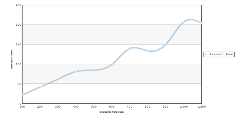
As a result of measurements, we get a certain number (median, minimum or other), but what can we say about our system (function) by one number? Imagine you are automating the process of obtaining this number and every day you will check it when you need to sound the alarm and look for the guilty? For example, here is a typical schedule of the same test every day.
Hidden text
If we want to write a performance report, with one number it will look empty. Therefore, we will definitely test for different parameters. Tests for different parameters will give us a beautiful graph and an idea of the scalability of the system.
Single parameter test
Consider a system with one numeric parameter. First of all, you need to select the parameter values. It does not make sense to choose numbers from different ranges, like [1, 100, 10000], you simply carry out 3 completely different incoherent tests and it will be impossible to find dependencies on such numbers. Imagine you want to build a graph, which numbers would you choose? Something similar to [X * 1, X * 2, X * 3, X * 4, X * 5,].
So, choose 5-10 (7 best) control points, for each point we make 3-7 measurements, take the minimum number for each point and build a graph.
Algorithm complexity
As you can see, the points are located exactly around the imaginary straight line. Now we come to the most interesting part of the measurements, we can determine the complexity of the algorithm based on the measurements. Determining the complexity of an algorithm based on tests is much easier for complex programs than analyzing the text of source programs. With the help of the test, you can even find special points when the difficulty changes, for example, the launch of Full GC.
Determining the complexity of the program on the test results is a direct task of the Regression analysis . Obviously, there is no general way to find a function only by a point; therefore, for the beginning, an assumption is made about some dependence, and then it is checked. In our case, and in most others, we assume that the function is a linear relationship.
Least squares method (linear model)
To search for linear dependence coefficients, there is a simple and optimal OLS method. The advantage of this method is that the formulas can be programmed in 10 lines and they are absolutely clear.
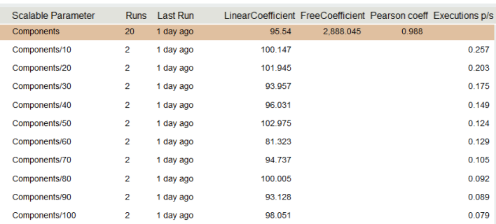
y = a + bx a = ([xy] - b[x])/[x^2] b = ([y] - a[x])/ n Let's present our calculations in the table.
In the highlighted line we see the linear coefficient of our model, it is equal to 95.54, the free coefficient is 2688. Now we can do a simple but not obvious focus, we can attach importance to these numbers. 95.54 is measured in milliseconds (as are our measurements), 95.54 is the time we spend on each component, and 2688 ms the time we spend on the system itself does not depend on the number of components. This method allowed us to allocate accurately enough the time of the external system, in this case the database, although it is ten times longer than the time of the 1st component. If we used the Time_with_N_component / N formula, we would have to measure for N> 1000 in order for the error to be less than 10%.
The linear coefficient of the model is the most important number of our measurements and oddly enough it is the most stable number of our measurements. The linear coefficient also makes it possible to adequately measure and interpret operations that occur in nanoseconds, and by separating the overhead of the system itself.
The graph shows the results of independent test launches at different times, which confirms the greater stability of the linear coefficient than individual tests.
Evaluation of the linearity of the model and the Pearson coefficient
Using the graph, we can visually see that our measurements really satisfy the linear model, but this method is far from accurate and we cannot automate it. In this case, the Pearson coefficient can help us. This method does show deviations from a straight line, but for 5-10 measurements it is clearly not enough. Below is an example of a clearly non-linear relationship, but the Pearson coefficient is quite high.
Returning to our table, knowing the ovehead of the system (free coefficient), we can calculate the linear coefficient for each measurement, which is done in the table. As we can see the numbers (100, 101, 93, 96, 102, 81, 94, 100, 93, 98) are rather randomly distributed around 95, which gives us weighty reasons to believe that the dependence is linear. Following the letter of mathematics, in fact, the deviations from the average value should satisfy the normal distribution, and to check the normal distribution, it suffices to check the Kolmogorov-Smirnov criterion, but we leave this for the sophisticated testers.
Oddly enough, not all dependencies are linear. The first thing that comes to mind is a quadratic dependence. In fact, quadratic dependency is very dangerous, it kills performance first slowly and then very quickly. Even if you have everything done for a fraction of a second for 1000 elements, then for 10,000 it will already be tens of seconds (multiplied by 100). Another example is sorting, which cannot be solved in linear time. Calculate how applicable the linear analysis method is for algorithms with complexity O (n * log n)
(10n log 10n )/ (n log n)= 10 + (10*log 10)/(log n) That is, for n> = 1000, the deviation will be within 10%, which is significant, but in some cases it can be applied, especially if the coefficient at log is large enough.
Consider an example of nonlinear dependence.
Nonlinear complexity of the algorithm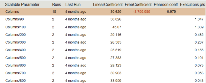
The first thing to note is negative overhead, for obvious reasons the system cannot have a negative time spent on preparation. The second, looking at the column of coefficients, you can notice a pattern, the linear coefficient falls, and then grows. This is reminiscent of a parabola chart.
Test with two or more parameters
Naturally, most systems do not consist of one parameter. For example, a program for reading from a table already consists of 2 parameters, columns and lines. Using parameterized tests, we can calculate what the cost of reading a row of 100 columns (let it be 100ms) and what are the costs of reading a column for 100 rows (let it be 150ms). 100 * 100ms! = 100 * 150ms and this is not a paradox, we just do not take into account that in the speed of reading lines there is already an overhead reading of 100 columns. That is, 100ms / 100 columns = 1ms - this is not the speed of reading a single cell! In fact, 2 measurements will not be enough to calculate the speed of reading a single cell. The general formula is as follows: where A is the cost per cell, B is one line, C is per column:
Time(row, column) = A * row * column + B * row + C * column + Overhead
Let's make a system of equations, taking into account the available values and one more necessary measurement:
Time(row, 100) = 100 * A * row + B * row + o = 100 * row + o. Time(row, 50) = 50 * A * row + B * row + o = 60 * row + o. Time(100, column) = 100 * B * column + C * column + o = 150 * column + o. 100 * A + B = 100. 50 * A + B = 55. 100 * B + C = 150. From here, we get A = 0.9 ms, B = 10 ms, C = 50 ms.
Of course, having a formula for the similarity of the LMIC for this case, all calculations would be simplified and automated. In general, the general LMIC does not apply to us, because a function that is linear in each of the arguments is not a multidimensional linear function (hyperplane in N-1 space). It is possible to use the gradient method of finding the coefficients, but this will not be an analytical method.
Multi-user tests and multi-core systems tests
Myth "throughput per core"
One of the favorite activities with performance tests is extrapolation. Especially people like to extrapolate to an area for which they cannot get values. For example, having 2 cores or 1 core in the system, I would like to extrapolate how the system behaved with 10 cores. And of course, the first wrong assumption is that the dependence is linear. For a normal definition of a linear relationship, it is necessary from 5 points, which of course is impossible to obtain on 2 cores.
Amdal's Law
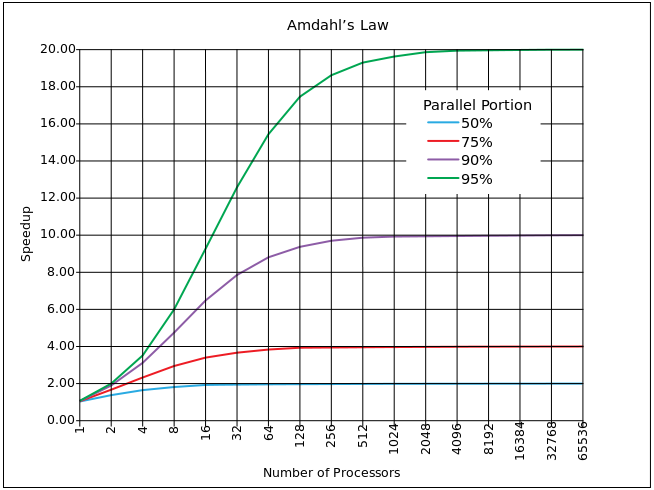
One of the closest approximations is the law of Amdal .
It is based on the calculation of the percentage of the parallelized code α (outside the synchronization block) and the synchronized code (1 - α). If one process takes time T on one core, then for multiple running tasks N time will be T '= T * α + (1-α) * N * T. On average, of course, N / 2, but Amdahl admits N. Parallel acceleration, respectively, S = N * T / T '= N / (α + (1-α) * N) = 1 / (α / N + (1 - α )).
Of course, the above graph is not so dramatic in reality (there is a logarithmic scale in X). However, a significant drawback of synchronization blocks is the asymptote. Relatively speaking, it is not possible by increasing the power to overcome the acceleration limit lim S = 1 / (1 - α). And this limit is quite hard, that is, for 10% of synchronized code, the limit is 10, for 5% (which is very good) the limit is 20.
The function has a limit, but it is constantly growing, and from this arises, at first glance, a strange task: to evaluate which hardware is optimal for our algorithm. In reality, it is quite difficult to increase the percentage of paralized. Let us return to the formula T '= T * α + (1-α) * N * T, optimal from the point of view of efficiency: if the kernel is idle, as much time as it will work. That is, T * α = (1-α) * N * T, hence we get N =
α / (1-α). For 10% - 9 cores, for 5% - 19 cores.
Communication of the number of users and the number of cores. Perfect schedule.
The model of acceleration of calculations is theoretically possible, but not always real. Consider a client-server situation where N clients are constantly running some task on the server, one by one, and we do not experience any costs of synchronizing the results, since the clients are not completely dependent! Keeping statistics for example introduces a synchronization element. Having a M-core machine, we expect the average query time T when N <M is the same, and when N> M the query time increases in proportion to the number of cores and users. Calculate throughput as the number of requests processed per second and get the following "ideal" schedule.
Perfect graphics

Experimental measurements
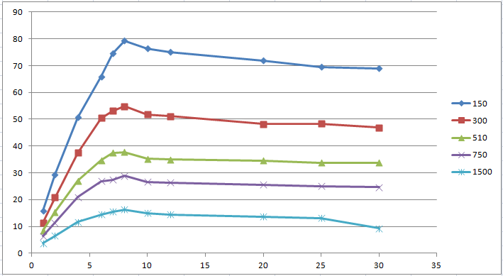
Naturally perfect graphics are achievable if we have 0% synchronized blocks (critical sections). Below are the actual measurements of one algorithm with different parameter values.
We can calculate the linear coefficient and build a graph. Also having a machine with 8 cores, it is possible to conduct a series of experiments for 2, 4, 8 cores. From the test results, you can see that a system with 4 cores and 4 users behaves just like a system with 8 cores and 4 users. Of course, this was expected, and gives us the opportunity to carry out only one series of tests for the machine with the maximum number of cores.
Experimental measurements using linear coefficient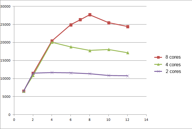
The measurement plots are close in value to the Amdal law, but still significantly different. Having measurements for 1, 2, 4, 8 cores, you can calculate the amount of non-parallelized code using the formula
Where NP is the number of cores, SU = Through NP core / Throughput 1 core. According to Amdal's law, this number should be constant, but in all dimensions this number falls, although not significantly (91% - 85%).
The throughput per core chart is not always a continuous line. For example, when there is a shortage of memory or when GC is running, deviations in throughput can be very significant.
Significant throughput fluctuations with Full GC
Behavioral test
Throughput
When measuring the load on multi-user systems, we introduced the definition of Throughput = NumberOfConcurrentUsers / AverageTimeResponse . To interpret the results. Throughput is the system capacity, how many users the system can serve at a time, and this definition is closely related to queuing theory . The difficulty of measuring throughput is that the value depends on the input stream. For example, in queuing systems, it is assumed that the waiting time for a response does not depend on how many applications are in the queue. In a simple software implementation, without a queue of requests, the time between all threads will be divided and, accordingly, the system will degrade. It is important to note that JMeter does not need to trust throughput measurements, it was noticed that Jmeter averages throughput between all test steps, which is not correct.
Consider the following case: with a load with 1 user, the system issues Throughput = 10, with 2 - Throughput = 5. This situation is quite possible, since the typical Throughput / User graph is a function that has one local (and global maximum).
Therefore, with an incoming stream of 1 user every 125ms, the system will process 8 users per second (input throughput).
With an incoming stream of 2 users every 125ms, the system will begin to collapse, since 8 (input throughput)> 5 (possible throughput).
Collapsing system
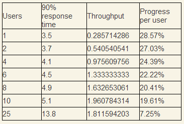
Consider an example of a collapsing system in more detail. After conducting the Throughput / Users test, we have the following results.
Users - the number of simultaneous users in the system; Progress per user - what amount of work as a percentage the user performs in one second. Mentally simulating the situation that 10 users come every second and begin to perform the same operation, the question is whether the system will be able to serve this stream.
In 1 second, 10 users on average will perform only 20% of their work, assuming that on average they perform all in 5. In the 2nd second there will already be 20 users in the system and they will share resources between 20 threads, which will further reduce percentage of work performed. We will continue the row until the moment when the first 10 users finish the work (theoretically they should finish it as the 1/2 / 1/3 + 1/4 row ... divergent).
It is quite obvious that the system will collapse, because after 80 seconds there will be 800 users in the system, and at this point only the first 10 users can finish.
This test shows that for any distribution of the incoming stream, if the incoming throughput (mathematical expectation) is greater than the maximum
measured throughput for the system, the system will begin to degrade and will fall at constant load. But the opposite is not true, in the 1st example, the maximum measured throughput (= 10)> incoming (8), but the system also cannot cope.
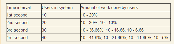
Stationary system
An interesting case is a workable system. Taking our measurements as a basis, we will test that every 1 second there are 2 new users. Since the minimum response time exceeds one second, at first the number of users will accumulate.
As we can see, the system will enter the stationary mode exactly at that point, the graphics when the measured throughput coincides with the input throughput. The average number of users in the system will be 10.
From this we can conclude that the Throughput / Users graph on the one hand represents the number of users processed per second (throughput) and the number of users in the system (users). The fall of the graph to the right of this point characterizes only the stability of the system in stressful situations and dependence on the nature of the incoming distribution. In any case, conducting tests Throughput / Users, it is not at all superfluous to conduct a behavioral test with approximate characteristics.
Amazing distribution
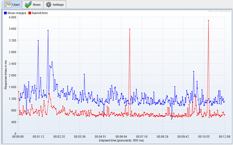
When conducting performance tests, there are almost always measurements that take much longer than expected. If the testing time is long enough, then you can observe the following picture. How to choose one number from all these dimensions?
Selection of statistics
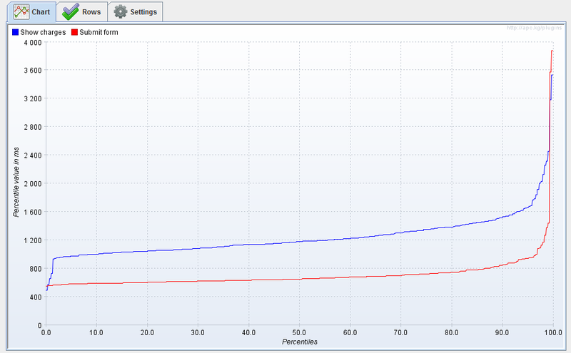
The simplest statistic is the average, but for the above reasons it is not quite stable, especially for a small number of measurements. To determine the quantile convenient to use the graph of the distribution function. Thanks to the wonderful JMeter plugin , we have this opportunity. After the first 10-15 measurements, the picture is usually not clear enough; therefore, a detailed study of the function will require 100 measurements.
First measurements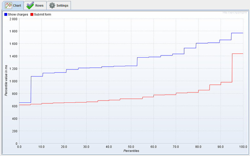
It is very simple to get the N-quantile from this graph; it is enough to take the value of the function at this point. The function shows a rather strange behavior around the minimum, but then it grows quite stably and only a sharp rise begins only near 95% of quantile.
Distribution?
Is this distribution analytical or known? To do this, you can plot the density distribution and try to see the known functions, fortunately there are not so many of them .
To be honest, this method did not bring any results, at first glance, similar distribution functions: Beta distribution, Maxwell distribution, turned out to be quite far from the statistics.
Minimum and exponential distribution
It is important to note that the range of our random variable is not at all [0, + ∞ [, but some [Min, + ∞ [. We cannot expect the program to execute faster than the theoretical minimum. If we assume that the measured minimum converges to the theoretical one and subtract this number from all the statistics, then a rather interesting regularity can be observed.
It turns out Minimum + StdDev = Mean (Average), and this is typical for all measurements. There is one known distribution of which, the expectation coincides with the variance, this exponential distribution. Although the distribution density graph is different at the beginning of the domain, the main quantiles completely coincide. Quite possibly, the random variable is the sum of the exponential distribution and the normal one, which fully explains the oscillations around the theoretical minimum point.
Variance and mean
Unfortunately, I was not able to find a theoretical justification for why the test results satisfy the exponential distribution. Most often, the exponential distribution appears in the problems of device failure time and even human lifetime. It is also unclear whether this is platform specific (Windows) or Java GC or any physical processes occurring in a computer.
, , 2 ( ) performance test , , peformance , 2 . — , — . , , , , , .
- , , . , , . 2 ( sleep), .
Source: https://habr.com/ru/post/171475/
All Articles