Briefly about hydrodynamics: equations of motion
Having written the previous post , historical and partly advertising (although potential applicants are unlikely to read this), one can proceed to the “essentially” conversation. Unfortunately, a high degree of popularity of the description is unlikely to be achieved, but still I will try not to arrange a course of dry lectures. Although, it was not possible to get rid of dryness, and the post was written as a result for exactly one month.
The current publication describes the basic equations of motion of an ideal and viscous fluid. If possible, their conclusion and physical meaning are briefly reviewed, and a few simplest examples of their exact solutions are described. Alas, these few examples of available analytically solutions of the Navier-Stokes equations are largely exhausted. Let me remind you that the Clay Institute carried the proof of the existence and smoothness of solutions to the problems of the millennium. Geniuses of the level of Perelman and higher - the task awaits you.
')
In, if I may say so, the "traditional" hydrodynamics that has developed historically, the foundation is the continuum model. It is distracted from the molecular structure of a substance, and describes the medium with several continuous field quantities: density, velocity (determined through the total impulse of molecules in a given volume element) and pressure. The continuum model assumes that there are still quite a lot of particles in any infinitely small volume (as they say, thermodynamically many — numbers that are close in order of magnitude to the Avogadro number — 10 23 pieces). Thus, the model is bounded below by the discreteness of the molecular structure of the liquid, which is completely irrelevant in problems of typical spatial scales.
However, this approach allows us to describe not only the water in a test tube or reservoir, and it turns out to be much more universal. Since our Universe on a large scale is almost homogeneous, then, oddly enough, since a certain scale, it is perfectly described as a continuous medium, taking into account, of course, self-gravity.
Other, more mundane applications of the continuum are the description of the properties of elastic bodies, plasma dynamics, and loose bodies. You can also describe the human fuel as a compressible fluid.
In parallel with the approach of a continuous medium, in recent years the kinetic model has been gaining momentum, based on the discretization of the medium into small particles interacting with each other (in the simplest case, as solid balls repelling in a collision). This approach arose primarily due to the development of computing technology, however, it didn’t exceed essential results in pure hydrodynamics, although it turned out to be extremely useful for problems of plasma physics, which is not homogeneous at the micro level, but contains electrons and positively charged ions. Well, again for modeling the universe .

The most elementary law. Suppose we have some completely arbitrary, but macroscopic volume of fluid V , bounded by surface F (see fig.). The mass of fluid inside it is determined by the integral:

And let nothing happen to the liquid inside it except for movement. That is, there are no chemical reactions and phase transitions, no tubes with pumps or black holes. Well, everything happens at low speeds and for small masses of matter, therefore, no theory of relativity, space curvature, liquid self-gravity (it becomes significant on a stellar scale). And let the volume itself and its boundaries be fixed. Then the only thing that can change the mass of fluid in our volume is its flow through the volume boundary (for definiteness, let the mass decrease in volume):

where vector j is the flow of matter through the border. The point, we recall, is the scalar product . Since the boundaries of the volume, as has been said, are fixed, then the time derivative can be introduced as an integral. And the right-hand side can be converted to the same, as on the left, integral over the volume according to the Gauss-Ostrogradsky theorem .
As a result, in both parts of the equality, the integral is obtained over the same completely arbitrary volume, which allows us to equate the integrands and go to the differential form of the equation:

Here (and further) the Hamilton vector operator is used. Figuratively speaking, this is a conditional vector whose components are differentiation operators according to the corresponding coordinates. It can be used to very briefly denote various kinds of operations on scalars, vectors, tensors of higher ranks and other mathematical evil spirits, the main ones of which are gradient , divergence and rotor . I will not dwell on them in detail, as it distracts from the main topic.
Finally, the flow of a substance is equal to the mass transferred through a single site per unit of time:

Finally, the law of conservation of mass (also called the continuity equation) for a continuum is:

This expression is the most common for a medium with variable density. In reality, the experiment indicates an extremely weak compressibility of the liquid and a practically constant density value, which with high accuracy allows the use of the law of mass conservation in the form of an incompressibility condition:

which works with no less good accuracy for gases, as long as the flow velocity is small compared with the sound one.
The entire relatively cumbersomewitchcraft process of converting integrals used above gives us not only the continuity equation. Exactly the same transformations make it possible to express the laws of conservation of momentum and energy, and ultimately obtain equations for the velocity of the fluid and for the transfer of heat in it. However, for the time being, we will not be in a great hurry, and will deal not only with the conservation of momentum, but even with the conservation of momentum in an ideal incompressible fluid — that is, Consider a model with no viscosity at all.
The reasoning is practically the same, only now we are not interested in mass, but in the total impulse of a liquid in the same volume V. It is equal to:

Under the same conditions as above, the volume impulse may vary due to:
The corresponding integrals (the order corresponds to the list) give the following relation:

Let's start to convert them. However, for this you need to use tensor analysis and rules for working with indices. More specifically, the Gauss-Ostrogradsky theorem is applied to the first and second integrals in a generalized form (it works not only for vector fields). And if you go to the differential form of the equation, you get the following:

A cross in a circle denotes a tensor product , in this case - vectors.
In principle, this is already the Euler equation, but it can be simplified a bit - after all, no one has repealed the law of conservation of mass. Opening here the brackets in the differential operators and then citing similar terms, we see that the three terms are safely assembled into the continuity equation , and therefore give a total of zero. The final equation is:

If we go to the reference system associated with a moving fluid (we will not focus on how this is done), we will see that the Euler equation expresses Newton's second law for a unit volume of the medium.
An ideal fluid, of course, is good (although it is still not exactly solved), but in many cases viscosity accounting is necessary. Even in the same convection, in the flow through the pipes. Without viscosity, water would flow out of our taps with cosmic velocities, and the slightest heterogeneity of temperature in water would lead to its extremely fast and rapid mixing. Therefore, let us take into account the resistance of the fluid to itself.
The Euler equation can be supplemented in various (but equivalent, of course) ways. We use the basic technique of tensor analysis - the index form of the equation. And while we also discard the external forces, so as not to be confused under the arms / under the legs / before the eyes (underline the necessary). In this scenario, everything, except the time derivative, can be collected in the form of the divergence of one such tensor:

By meaning, this is the density of the momentum flux in a liquid. Viscous forces must be added to it in the form of one more tensor term. Since they clearly lead to a loss of energy (and momentum), they must be subtracted:

Going back to the equation with such a tensor, we obtain the generalized equation of motion of a viscous fluid:

It admits any law for viscosity.
It is considered to be obvious that the resistance depends on the speed of movement. Viscosity, as the transfer of momentum between parts of a fluid with different velocities, depends on the velocity gradient (but not on the velocity itself - the principle of relativity interferes with this). If we confine ourselves to the decomposition of this dependence into linear terms, we get this eerie object:

in which the value before the derivative contains 81 coefficient. However, using a number of perfectly reasonable assumptions about the homogeneity and isotropy of a fluid, from 81 coefficients you can go to just two, and in the general case for a compressible medium, the viscous stress tensor is equal to:

where η (eta) is the shear viscosity, and ζ (zeta or zeta) is the bulk viscosity. If the medium is also incompressible, then a single shear viscosity coefficient is sufficient, since the second term goes away. Such a law of viscosity

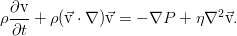
is called the Navier law, and the equation of motion obtained by substituting it is the Navier-Stokes equation:
The main problem of hydrodynamics is the lack of exact solutions to its equations. No matter how they fought against this, it’s still not possible to obtain truly universal results, and I remind you that the question of the existence and smoothness of solutions of the Navier-Stokes equations is on the Clay Institute’s millennium problem list.
However, despite such sad facts, there are some results. Far from all will be presented here, but only the simplest cases.
Of particular interest are flows in which the fluid does not swirl. For such a situation, it is possible to refuse to consider the vector velocity field, since it is expressed in terms of the gradient of the scalar function - the potential. The potential, on the other hand, satisfies the well-studied Laplace equation, whose solution is completely determined by what is given on the boundaries of the considered region:

Moreover, in the absence of viscosity from the Euler equation, pressure can be unambiguously expressed, which is quite remarkable and leads us to complete solution of the problem. Oh, if it had always been like this ... then hydrodynamics, probably, would not have existed as a modern and relevant industry.
Additionally, you can simplify the problem by assuming that the fluid flow is two-dimensional — say, everything moves in the (x, y) plane, and not a single particle moves along the z axis. It can be shown that in this case the speed can also be replaced by a scalar function (this time by the current function):

which, in the case of a potential flow, satisfies the Cauchy-Lagrange conditions from the theory of functions of a complex variable, and use the corresponding mathematical apparatus. Fully coincident with the electrostatic apparatus. The theory of potential flows is developed at a high level, and, in principle, well describes a wide range of problems.
Solutions for a viscous fluid are most often obtained when the nonlinear term falls out of the Navier-Stokes equation due to the symmetry properties of the problem.
The most elementary task. A channel with a fixed lower and a movable upper wall that moves uniformly at a certain speed. At the boundaries, the fluid sticks to them, so that the velocity of the fluid is equal to the velocity of the boundary. This result is an experimental fact, and somehow even the authors of the first experiments are not mentioned, simply - by a combination of experiments.
In such a situation, the equation of the form v '' = 0 will remain from the Navier-Stokes equation, and therefore the velocity profile in the channel will be linear:

This task is almost basic for the theory of lubrication, because allows you to directly determine the force that you want to attach to the upper wall for its movement with a specific speed.
The second elementary is the laminar flow in the channel. Or in the pipe. The result is the same - the velocity profile is parabolic:

Based on the Poiseuille solution, it is possible to determine the flow rate through the channel section, but, true, only with laminar flow and smooth walls. On the other hand, for a turbulent flow and rough walls there are no exact solutions, but only approximate empirical laws.
Here - almost as in the Poiseuille problem, only the upper boundary of the fluid will be free. If we assume that no waves run over it, and there is generally no friction from above, then the velocity profile will be practically the lower half of the previous figure. However, if from the resulting dependence we calculate the flow velocity for an average lowland river, it will be about 10 km / s, and the water should spontaneously go into space. The low flow rates observed in nature are associated with developed vorticity and flow turbulence, which effectively increase the viscosity of water by about 1 million times.
In the next post, we plan to talk about the law of energy conservation and the corresponding equations of heat transfer during the flow of a liquid.
The current publication describes the basic equations of motion of an ideal and viscous fluid. If possible, their conclusion and physical meaning are briefly reviewed, and a few simplest examples of their exact solutions are described. Alas, these few examples of available analytically solutions of the Navier-Stokes equations are largely exhausted. Let me remind you that the Clay Institute carried the proof of the existence and smoothness of solutions to the problems of the millennium. Geniuses of the level of Perelman and higher - the task awaits you.
Continuum concept
')
In, if I may say so, the "traditional" hydrodynamics that has developed historically, the foundation is the continuum model. It is distracted from the molecular structure of a substance, and describes the medium with several continuous field quantities: density, velocity (determined through the total impulse of molecules in a given volume element) and pressure. The continuum model assumes that there are still quite a lot of particles in any infinitely small volume (as they say, thermodynamically many — numbers that are close in order of magnitude to the Avogadro number — 10 23 pieces). Thus, the model is bounded below by the discreteness of the molecular structure of the liquid, which is completely irrelevant in problems of typical spatial scales.
However, this approach allows us to describe not only the water in a test tube or reservoir, and it turns out to be much more universal. Since our Universe on a large scale is almost homogeneous, then, oddly enough, since a certain scale, it is perfectly described as a continuous medium, taking into account, of course, self-gravity.
Other, more mundane applications of the continuum are the description of the properties of elastic bodies, plasma dynamics, and loose bodies. You can also describe the human fuel as a compressible fluid.
In parallel with the approach of a continuous medium, in recent years the kinetic model has been gaining momentum, based on the discretization of the medium into small particles interacting with each other (in the simplest case, as solid balls repelling in a collision). This approach arose primarily due to the development of computing technology, however, it didn’t exceed essential results in pure hydrodynamics, although it turned out to be extremely useful for problems of plasma physics, which is not homogeneous at the micro level, but contains electrons and positively charged ions. Well, again for modeling the universe .
The continuity equation. Mass conservation law
The most elementary law. Suppose we have some completely arbitrary, but macroscopic volume of fluid V , bounded by surface F (see fig.). The mass of fluid inside it is determined by the integral:
And let nothing happen to the liquid inside it except for movement. That is, there are no chemical reactions and phase transitions, no tubes with pumps or black holes. Well, everything happens at low speeds and for small masses of matter, therefore, no theory of relativity, space curvature, liquid self-gravity (it becomes significant on a stellar scale). And let the volume itself and its boundaries be fixed. Then the only thing that can change the mass of fluid in our volume is its flow through the volume boundary (for definiteness, let the mass decrease in volume):
where vector j is the flow of matter through the border. The point, we recall, is the scalar product . Since the boundaries of the volume, as has been said, are fixed, then the time derivative can be introduced as an integral. And the right-hand side can be converted to the same, as on the left, integral over the volume according to the Gauss-Ostrogradsky theorem .
As a result, in both parts of the equality, the integral is obtained over the same completely arbitrary volume, which allows us to equate the integrands and go to the differential form of the equation:
Here (and further) the Hamilton vector operator is used. Figuratively speaking, this is a conditional vector whose components are differentiation operators according to the corresponding coordinates. It can be used to very briefly denote various kinds of operations on scalars, vectors, tensors of higher ranks and other mathematical evil spirits, the main ones of which are gradient , divergence and rotor . I will not dwell on them in detail, as it distracts from the main topic.
Finally, the flow of a substance is equal to the mass transferred through a single site per unit of time:
Finally, the law of conservation of mass (also called the continuity equation) for a continuum is:
This expression is the most common for a medium with variable density. In reality, the experiment indicates an extremely weak compressibility of the liquid and a practically constant density value, which with high accuracy allows the use of the law of mass conservation in the form of an incompressibility condition:
which works with no less good accuracy for gases, as long as the flow velocity is small compared with the sound one.
Euler equation. Momentum conservation law
The entire relatively cumbersome
The reasoning is practically the same, only now we are not interested in mass, but in the total impulse of a liquid in the same volume V. It is equal to:
Under the same conditions as above, the volume impulse may vary due to:
- convective transport - i.e. impulse "leaks" along with speed across the border
- pressure surrounding fluid elements
- just due to external forces, for example - from gravity.
The corresponding integrals (the order corresponds to the list) give the following relation:
Let's start to convert them. However, for this you need to use tensor analysis and rules for working with indices. More specifically, the Gauss-Ostrogradsky theorem is applied to the first and second integrals in a generalized form (it works not only for vector fields). And if you go to the differential form of the equation, you get the following:
A cross in a circle denotes a tensor product , in this case - vectors.
In principle, this is already the Euler equation, but it can be simplified a bit - after all, no one has repealed the law of conservation of mass. Opening here the brackets in the differential operators and then citing similar terms, we see that the three terms are safely assembled into the continuity equation , and therefore give a total of zero. The final equation is:
If we go to the reference system associated with a moving fluid (we will not focus on how this is done), we will see that the Euler equation expresses Newton's second law for a unit volume of the medium.
Viscosity accounting. Navier-Stokes equation
An ideal fluid, of course, is good (although it is still not exactly solved), but in many cases viscosity accounting is necessary. Even in the same convection, in the flow through the pipes. Without viscosity, water would flow out of our taps with cosmic velocities, and the slightest heterogeneity of temperature in water would lead to its extremely fast and rapid mixing. Therefore, let us take into account the resistance of the fluid to itself.
The Euler equation can be supplemented in various (but equivalent, of course) ways. We use the basic technique of tensor analysis - the index form of the equation. And while we also discard the external forces, so as not to be confused under the arms / under the legs / before the eyes (underline the necessary). In this scenario, everything, except the time derivative, can be collected in the form of the divergence of one such tensor:
By meaning, this is the density of the momentum flux in a liquid. Viscous forces must be added to it in the form of one more tensor term. Since they clearly lead to a loss of energy (and momentum), they must be subtracted:
Going back to the equation with such a tensor, we obtain the generalized equation of motion of a viscous fluid:
It admits any law for viscosity.
It is considered to be obvious that the resistance depends on the speed of movement. Viscosity, as the transfer of momentum between parts of a fluid with different velocities, depends on the velocity gradient (but not on the velocity itself - the principle of relativity interferes with this). If we confine ourselves to the decomposition of this dependence into linear terms, we get this eerie object:
in which the value before the derivative contains 81 coefficient. However, using a number of perfectly reasonable assumptions about the homogeneity and isotropy of a fluid, from 81 coefficients you can go to just two, and in the general case for a compressible medium, the viscous stress tensor is equal to:
where η (eta) is the shear viscosity, and ζ (zeta or zeta) is the bulk viscosity. If the medium is also incompressible, then a single shear viscosity coefficient is sufficient, since the second term goes away. Such a law of viscosity
is called the Navier law, and the equation of motion obtained by substituting it is the Navier-Stokes equation:
Exact solutions
The main problem of hydrodynamics is the lack of exact solutions to its equations. No matter how they fought against this, it’s still not possible to obtain truly universal results, and I remind you that the question of the existence and smoothness of solutions of the Navier-Stokes equations is on the Clay Institute’s millennium problem list.
However, despite such sad facts, there are some results. Far from all will be presented here, but only the simplest cases.
Potential currents
Of particular interest are flows in which the fluid does not swirl. For such a situation, it is possible to refuse to consider the vector velocity field, since it is expressed in terms of the gradient of the scalar function - the potential. The potential, on the other hand, satisfies the well-studied Laplace equation, whose solution is completely determined by what is given on the boundaries of the considered region:
Moreover, in the absence of viscosity from the Euler equation, pressure can be unambiguously expressed, which is quite remarkable and leads us to complete solution of the problem. Oh, if it had always been like this ... then hydrodynamics, probably, would not have existed as a modern and relevant industry.
Additionally, you can simplify the problem by assuming that the fluid flow is two-dimensional — say, everything moves in the (x, y) plane, and not a single particle moves along the z axis. It can be shown that in this case the speed can also be replaced by a scalar function (this time by the current function):
which, in the case of a potential flow, satisfies the Cauchy-Lagrange conditions from the theory of functions of a complex variable, and use the corresponding mathematical apparatus. Fully coincident with the electrostatic apparatus. The theory of potential flows is developed at a high level, and, in principle, well describes a wide range of problems.
Simple viscous flow
Solutions for a viscous fluid are most often obtained when the nonlinear term falls out of the Navier-Stokes equation due to the symmetry properties of the problem.
Quat slip
The most elementary task. A channel with a fixed lower and a movable upper wall that moves uniformly at a certain speed. At the boundaries, the fluid sticks to them, so that the velocity of the fluid is equal to the velocity of the boundary. This result is an experimental fact, and somehow even the authors of the first experiments are not mentioned, simply - by a combination of experiments.
In such a situation, the equation of the form v '' = 0 will remain from the Navier-Stokes equation, and therefore the velocity profile in the channel will be linear:
This task is almost basic for the theory of lubrication, because allows you to directly determine the force that you want to attach to the upper wall for its movement with a specific speed.
Poiseuille flow
The second elementary is the laminar flow in the channel. Or in the pipe. The result is the same - the velocity profile is parabolic:
Based on the Poiseuille solution, it is possible to determine the flow rate through the channel section, but, true, only with laminar flow and smooth walls. On the other hand, for a turbulent flow and rough walls there are no exact solutions, but only approximate empirical laws.
The flow of a fluid layer on an inclined plane
Here - almost as in the Poiseuille problem, only the upper boundary of the fluid will be free. If we assume that no waves run over it, and there is generally no friction from above, then the velocity profile will be practically the lower half of the previous figure. However, if from the resulting dependence we calculate the flow velocity for an average lowland river, it will be about 10 km / s, and the water should spontaneously go into space. The low flow rates observed in nature are associated with developed vorticity and flow turbulence, which effectively increase the viscosity of water by about 1 million times.
In the next post, we plan to talk about the law of energy conservation and the corresponding equations of heat transfer during the flow of a liquid.
Source: https://habr.com/ru/post/171327/
All Articles