Introduction to Bayesian Methods

As an introduction

At present, Bayesian methods are widely used and are widely used in various fields of knowledge. However, unfortunately, not many people have an idea of ​​what it is and why it is needed. One of the reasons is the lack of a large amount of literature in Russian. Therefore, here I will try to state their principles as simply as I can, starting from the very beginning (I apologize if this seems too simple to someone).

In the future, I would like to go directly to Bayesian analysis and talk about the processing of real data and, in my opinion, an excellent alternative to the R language (it was written a little about it here ) - Python with the pymc module. Personally, Python seems to me much more understandable and logical than R with JAGS and BUGS packages, besides Python gives much more freedom and flexibility (although Python has its own difficulties, but they are surmountable, and in simple analysis are not often ).

A bit of history

As a brief historical background, I will say that the Bayesian formula was already published in 1763, 2 years after the death of its author, Thomas Bayes. However, the methods using it were really widespread only by the end of the twentieth century. This is explained by the fact that the calculations require certain computational costs, and they became possible only with the development of information technologies.

On probability and the Bayes theorem

The Bayes formula and all subsequent statements require an understanding of probability. More information about the probability can be read on Wikipedia .
In practice, the probability of an event occurring is the frequency of occurrence of this event, that is, the ratio of the number of observations of an event to the total number of observations with a large (theoretically infinite) total number of observations.
Consider the following experiment: we call any number from the segment [0, 1] and look at what this number will be between, for example, 0.1 and 0.4. As you might guess, the probability of this event will be equal to the ratio of the length of the segment [0.1, 0.4] to the total length of the segment [0, 1] (in other words, the ratio of the “number” of possible equiprobable values ​​to the total “number” of values), that is (0.4 - 0.1) / (1 - 0) = 0.3, that is, the probability of hitting the [0.1, 0.4] segment is 30%.
')
Now look at the square [0, 1] x [0, 1].


Suppose we have to call pairs of numbers (x, y), each of which is greater than zero and less than one. The probability that x (the first number) will be within the interval [0.1, 0.4] (shown in the first picture as a blue area, at the moment the second number y is not important for us) is equal to the ratio of the area of ​​the blue area to the area of ​​the entire square, there is (0.4 - 0.1) * (1 - 0) / (1 * 1) = 0.3, that is, 30%. Thus, we can write that the probability that x belongs to the segment [0.1, 0.4] is equal to p (0.1 <= x <= 0.4) = 0.3 or, for short, p (X) = 0.3.
If we now look at y, then, similarly, the probability that y is inside the segment [0.5, 0.7] is equal to the ratio of the area of ​​the green area to the area of ​​the entire square p (0.5 <= y <= 0.7) = 0.2, or for brevity p (Y) = 0.2.
Now let's see what you can learn about the values ​​of x and y at the same time.
If we want to know what is the probability that both x and y are in the corresponding given segments, then we need to calculate the ratio of the dark area (the intersection of the green and blue areas) to the area of ​​the whole square: p (X, Y) = (0.4 - 0.1 ) * (0.7 - 0.5) / (1 * 1) = 0.06.

And now let's say we want to know what is the probability that y is in the interval [0.5, 0.7], if x is already in the interval [0.1, 0.4]. That is, in fact, we have a filter and when we call pairs (x, y), we immediately discard those pairs that do not satisfy the condition for finding x in a given interval, and then from the filtered pairs we consider those for which y satisfies our condition and consider the probability as the ratio of the number of pairs for which y lies in the above segment to the total number of filtered pairs (that is, for which x lies in the interval [0.1, 0.4]). We can write this probability as p (Y | X). Obviously, this probability is equal to the ratio of the area of ​​the dark area (the intersection of the green and blue areas) to the area of ​​the blue area. The area of ​​the dark area is (0.4 - 0.1) * (0.7 - 0.5) = 0.06, and the area of ​​the blue (0.4 - 0.1) * (1 - 0) = 0.3, then their ratio is 0.06 / 0.3 = 0.2. In other words, the probability of finding y on the interval [0.5, 0.7], while x already belongs to the segment [0.1, 0.4] is equal to p (Y | X) = 0.2.
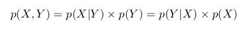
It can be noted that, in view of the foregoing and all the above notation, we can write the following expression
p (Y | X) = p (X, Y) / p (X)

Let us briefly reproduce all the previous logic with respect to p (X | Y): we call pairs (x, y) and filter those for which y lies between 0.5 and 0.7, then the probability that x lies in the interval [0.1, 0.4 ] provided that y belongs to the segment [0.5, 0.7] is equal to the ratio of the area of ​​the dark area to the area of ​​green:
p (X | Y) = p (X, Y) / p (Y)

In the two formulas above, we see that the term p (X, Y) is the same, and we can exclude it:

We can rewrite the last equality as


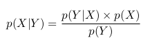
This is the Bayes theorem.
It is also interesting to note that p (Y) is actually p (X, Y) for all values ​​of X. That is, if we take a dark area and stretch it so that it covers all values ​​of X, it will exactly repeat the green area , which means that it will be equal to p (Y). In the language of mathematics, this would mean the following:
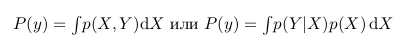
Then we can rewrite the Bayes formula as follows:

Application of the Bayes theorem

Let's consider the following example. Take a coin and throw it 3 times. With the same probability we can get the following results (O - Eagle, P - Tails): LLC, OOR, ORO, ORR, ROO, ROR, PPO, PPP.

We can calculate how many eagles fell in each case and how many shifts were all heads-tails, tails-heads:


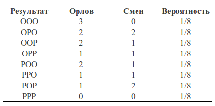
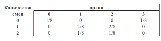
We can consider the number of eagles and the number of changes as two random variables. Then the probability table will have the following form:


Now we can see the Bayes formula in action.
But before we draw an analogy with the square, which we considered earlier.
You can see that p (1O) is the sum of the third column (the “blue region” of the square) and is equal to the sum of all cell values ​​in this column: p (1O) = 2/8 + 1/8 = 3/8
p (1) is the sum of the third row (the "green area" of the square) and, similarly, is equal to the sum of all cell values ​​in this row p (1) = 2/8 + 2/8 = 4/8
The probability that we got one eagle and one shift is equal to the intersection of these areas (that is, the value in the cage of the intersection of the third column and the third row) p (1C, 1O) = 2/8
Then, following the formulas described above, we can calculate the probability of getting one shift, if we got one eagle in three throws:
p (1 | 1) = p (1, 1) / p (1) = (2/8) / (3/8) = 2/3
or the probability of getting one eagle, if we got one shift:
p (1 | 1) = p (1, 1) / p (1) = (2/8) / (4/8) = 1/2
If we calculate the probability of getting one shift in the presence of one eagle p (1 | 1) through the Bayes formula, we get:
p (1 | 1) = p (1 | 1) * p (1) / p (1) = (2/3) * (3/8) / (4/8) = 1/2
What we got higher.

But what practical value does the above example have?
The fact is that when we analyze real data, we are usually interested in some parameter of this data (for example, mean, variance, etc.). Then we can draw the following analogy with the above table of probabilities: let the rows be our experimental data (we denote them Data), and the columns the possible values ​​of the parameter of interest to us this data (we denote it ). Then we are interested in the probability of obtaining a certain parameter value based on the available data. .
We can apply Baeys formula and write the following:

And remembering the formula with the integral, we can write the following:


That is, in fact, as a result of our analysis, we have the probability as a function of a parameter. Now we can, for example, maximize this function and find the most likely parameter value, calculate the variance and average value of the parameter, calculate the boundaries of the segment within which the parameter of interest lies with a probability of 95%, etc.

Probability called a posteriori probability. And in order to calculate it we need to have
- the likelihood function and - prior probability.
The likelihood function is determined by our model. That is, we create a data collection model that depends on the parameter we are interested in. For example, we want to interpolate data using the straight line y = a * x + b (thus, we assume that all data have a linear relationship with Gaussian noise superimposed on it with known dispersion). Then a and b are our parameters, and we want to know their most probable values, and the likelihood function is Gauss with an average, given by a straight line equation, and a given dispersion.
A priori probability includes information that we know prior to analysis. For example, we know for sure that the straight line should have a positive slope, or that the value at the point of intersection with the x axis should be positive - all this and not only we can incorporate into our analysis.
As you can see, the denominator fraction is an integral (or in the case when the parameters can take only certain discrete values, the sum) of the numerator over all possible values ​​of the parameter. In practice, this means that the denominator is a constant and serves to normalize the a posteriori probability (that is, the a posteriori probability integral is equal to unity).

At this point I would like to finish my post (continued here ). I will be glad to your comments.