Optical flux calculation using the Lucas-Canada method. Theory

In computer vision and image processing systems, it is often necessary to determine the movement of objects in three-dimensional space using an optical sensor, that is, a video camera. Having a sequence of frames at the entrance, it is necessary to recreate the three-dimensional space captured on them and the changes that occur with it over time. It sounds difficult, but in practice it is often enough to find the displacements of two-dimensional projections of objects in the plane of the frame.



If we want to know how much an object has shifted relative to its position on the previous frame during the time elapsed between the fixation of frames, then most likely we will first recall the optical flow. To find the optical flow, you can safely use the finished tested and optimized implementation of one of the algorithms, for example, from the OpenCV library. At the same time, however, it is very harmless to understand the theory, so I invite all those interested to look inside one of the most popular and well-studied methods. In this article, there is no code and practical advice, but there are formulas and a number of mathematical conclusions.



There are several approaches to determining offsets between two adjacent frames. For example, for each small fragment (say, 8 by 8 pixels) of one frame, it is possible to find the most similar fragment in the next frame. In this case, the difference between the coordinates of the original and the found fragments will give us an offset. The main difficulty here is how to quickly find the desired fragment, without going through the entire frame pixel by pixel. Various implementations of this approach somehow solve the problem of computational complexity. Some are so successful that they apply, for example, in common video compression standards. The price for speed is of course quality. We will consider a different approach, which allows us to obtain offsets not for fragments, but for each individual pixel, and is applied when speed is not so critical. The term “optical flow” is often associated with it in the literature.



This approach is often called differential, because it is based on the calculation of partial derivatives in the horizontal and vertical directions of the image. As we shall see, the derivatives alone are not enough to determine the displacements. That is why, on the basis of one simple idea, a great variety of methods appeared, each of which uses some of its mathematical dance with a tambourine to achieve the goal. Focus on the Lucas-Kanade method, proposed in '81 by Bruce Lucas and Takeo Canada.

')

Lucas-Canada method

The basis of all further reasoning is one very important and not very fair assumption: Suppose that the pixel values ​​are transferred from one frame to the next without any changes . Thus, we assume that the pixels belonging to the same object may move in some direction, but their value will remain unchanged. Of course, this assumption has little to do with reality, because global conditions of illumination and illumination of the moving object itself may vary from frame to frame. A lot of problems associated with this assumption, but, oddly enough, despite everything, it works quite well in practice.



In mathematical language, this assumption can be written as: . Where I is the function of the brightness of pixels from the position on the frame and the time. In other words, x and y are the coordinates of a pixel in the frame plane, and Is the offset, and t is the frame number in the sequence. We will agree that a single interval of time passes between two adjacent frames.

One-dimensional case

To begin, consider the one-dimensional case. Imagine two one-dimensional frames 1 pixel high and 20 pixels wide (right figure). In the second frame, the image is slightly shifted to the right. This is the offset we want to find. To do this, we represent the same frames as functions (figure on the left). At the input, the position of the pixel, at the output - its intensity. In such a view, the desired displacement (d) can be seen even more clearly. In accordance with our assumption it's just biased that is, we can say that .



note that and if you wish, you can write in the general form: ; where y and t are fixed and equal to zero.



For each coordinate, we know the values and at this point, moreover, we can calculate their derivatives. We associate the known values ​​with the offset d. To do this, we write the decomposition in the Taylor series for :







We make the second important assumption: Suppose that fairly well approximated by the first derivative . Having made this assumption, we drop everything after the first derivative:







How correct is this? In general, not very, here we lose exactly, unless our function / image is strictly linear, as in our artificial example. But this greatly simplifies the method, and to achieve the required accuracy, you can make a consistent approximation, which we will consider later.



We are almost there. The offset d is our desired quantity, so something needs to be done with . As we agreed earlier, so just rewrite:







I.e:

Two-dimensional case

We now turn from one-dimensional to two-dimensional case. We write the decomposition in the Taylor series for and immediately discard all higher derivatives. Instead of the first derivative, a gradient appears:







Where - displacement vector.

In accordance with the assumption made . Note that this expression is equivalent to . That's what we need. Rewrite:











Since there is a unit time interval between two frames, it can be said that is nothing but a time derivative.

Rewrite:







Rewrite again, revealing a gradient:







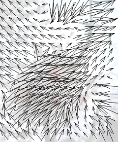
We have obtained an equation that tells us that the sum of the partial derivatives should be zero. The only problem is that we have one equation, and two unknowns in it: and . At this moment, the flight of fantasy and diversity of approaches begins.



Make the third assumption: Suppose that the neighboring pixels are shifted by the same distance . Take a fragment of the image, say 5 by 5 pixels, and agree that for each of the 25 pixels and are equal. Then instead of one equation we get 25 equations at once! It is obvious that in the general case the system has no solution, therefore we will look for such and that minimize the error:







Here g is the function that determines the weights for the pixels. The most common option is a two-dimensional Gaussian, which gives the greatest weight to the central pixel and less and less as the distance from the center.



To find the minimum let's use the least squares method, find its partial derivatives with respect to and :











Rewrite in a more compact form and equate to zero:











Rewrite these two equations in matrix form:







Where















If the matrix M is reversible (has rank 2), we can calculate and that minimize the error E:







That's all. We know the approximate pixel offset between two adjacent frames.



Since neighboring pixels also take part in finding the offset of each pixel, when implementing this method, it is advisable to preliminarily calculate the frame derivatives horizontally and vertically.

Method disadvantages

The method described above is based on three significant assumptions, which, on the one hand, give us a fundamental opportunity to determine the optical flux, but, on the other hand, introduce an error. The good news for perfectionists is that we only need one assumption to simplify the method, and we can deal with its consequences. We assumed that the first derivative would be enough for us to approximate the bias. In the general case, this is certainly not the case (left figure). To achieve the required accuracy, the offset for each pair of frames (let's call them and ) can be calculated iteratively. In the literature, this is called warping. In practice, this means that by calculating the offsets at the first iteration, we move each pixel of the frame in the opposite direction so that this offset is compensated. At the next iteration instead of the original frame we will use its distorted version . And so on, until at the next iteration all the resulting offsets will not be less than the specified threshold value. We get the total offset for each specific pixel as the sum of its offsets at all iterations.



By its nature, this method is local, that is, when determining the offset of a particular pixel, only the area around this pixel is taken into account - a local neighborhood. As a consequence, it is impossible to determine the displacements within sufficiently large (larger than the size of the local neighborhood) of uniformly colored frame areas. Fortunately, on real frames such areas are not often found, but this feature still introduces an additional deviation from the true offset.



Another problem is that some textures in the image give a degenerate matrix M, for which the inverse matrix cannot be found. Accordingly, for such textures we will not be able to determine the offset. That is, the movement seems to be there, but it is not clear which way. In general, not only the method considered suffers from this problem. Even the human eye perceives such a movement is not uniquely ( Barber pole ).

Conclusion

We have analyzed the theoretical foundations of one of the differential methods for finding the optical flow. There are many other interesting methods, some of which, as of today, give more reliable results. However, the method of Lucas-Canada, with its good performance remains simple enough to understand, and therefore well suited for familiarizing with the mathematical foundations.



Although the problem of finding the optical flux has been studied for several decades, methods are still being improved. The work continues in view of the fact that, upon close examination, the problem turns out to be very difficult, and the quality and definition of displacements in video and image processing determines the stability and efficiency of many other algorithms.



On this pathetic note, let me round out and go to the sources and useful links.

Sources and references

1. Optical Flow Estimation. David J. Fleet, Yair Weiss. - Detailed article, which contains a detailed description of not only the method of Lucas-Canada, but also other differential methods.

2. Image and Video Compression for Multimedia Engineering: Fundamentals, Algorithms, and Standards. Yun Q. Shi, Huifang Sun - Tutorial on compressing video and images, but also contains a good overview of the background.

3. Image Processing On Line - A large number of actual image processing algorithms. Best of all, the algorithms are equipped with an online demo .