Kalman filter
On the Internet, including on Habré, you can find a lot of information about the Kalman filter. But it is hard to find an easily digestible conclusion of the formulas themselves. Without conclusion, all this science is perceived as a kind of shamanism, formulas look like a faceless set of symbols, and most importantly, many simple statements lying on the surface of the theory are beyond comprehension. The purpose of this article will be to tell about this filter in the most accessible language.
Kalman Filter is the most powerful data filtering tool. Its main principle is that when filtering information is used on the physics of the phenomenon itself. For example, if you are filtering data from the machine’s speedometer, the inertia of the machine gives you the right to perceive too fast speed jumps as a measurement error. The Kalman filter is interesting because in some sense this is the best filter. We will discuss in more detail below what exactly the words “the best” mean. At the end of the article I will show that in many cases the formulas can be simplified to such an extent that almost nothing will remain of them.
Likbez
Before getting acquainted with the Kalman filter, I propose to recall some simple definitions and facts from probability theory.
Random value
When they say that a random variable is given
 , they mean that this value can take random values. It takes different values with different probabilities. When you roll, say, a bone, a discrete set of values will appear:
 In the case of a continuous set of values, a random variable characterizes the probability density

')
Quite often in life, random variables are distributed in Gauss, when the probability density is

We see that function
Once we started talking about the Gaussian distribution, it would be a sin not to mention where it came from. As well as numbers
Let there be a random variable
Average value
The average value of a random variable is what we will get in the limit if we carry out a lot of experiments and calculate the arithmetic average of the values that have been dropped. Mean value is denoted differently: mathematicians like to denote by
For example, for Gaussian distribution
Dispersion
In the case of the Gauss distribution, we clearly see that the random variable prefers to fall out in a certain neighborhood of its mean value.
Once again admire the Gaussian distribution
As can be seen from the graph, the characteristic variation of the values of the order
An easier way (simpler in terms of calculations) is to find
For example, for the Gaussian distribution
In fact, there is a small fraud. The fact is that in the definition of a Gaussian distribution, under the exponent is the expression
Independent random variables
Random variables are dependent and not. Imagine that you are throwing a needle on a plane and recording the coordinates of its both ends. These two coordinates are dependent, they are connected by the condition that the distance between them is always equal to the length of the needle, although they are random variables.
Random variables are independent if the result of the fallout of the first one is completely independent of the result of the fallout of the second one. If random values
Evidence
For example, having blue eyes and graduating from school with a gold medal is independent random values. If the blue-eyed, say  and gold medalists
  the blue eyed medalists
  This example tells us that if random variables
  and given by their probability densities
  and
and  , the independence of these quantities is expressed in the fact that the probability density
  (the first value fell
  and the second
  ) is according to the formula:
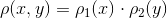
It immediately follows that:
As you can see, the proof is carried out for random variables that have a continuous spectrum of values and are given by their probability density. In other cases, the idea of proof is similar.
It immediately follows that:
As you can see, the proof is carried out for random variables that have a continuous spectrum of values and are given by their probability density. In other cases, the idea of proof is similar.
Kalman filter
Formulation of the problem
Denote by
Let's start with a simple example that will lead us to the formulation of a common task. Imagine that we have a radio-controlled machine that can only go back and forth. Knowing the weight of the car, the shape, the road surface, etc., we calculated how the control joystick affects the speed of movement.

Then the coordinate of the machine will change according to the law:
In real life, we cannot take into account in our calculations the small perturbations acting on the car (wind, bumps, pebbles on the road), therefore the real speed of the car will differ from the calculated one. A random variable will be added to the right side of the written equation.
We have a GPS-mounted sensor that tries to measure the true coordinate
The challenge is that, knowing the wrong sensor readings
In the formulation of the general problem, for the coordinate
 (one)
(one)Let's discuss in detail what we know:
- This is a known value that controls the evolution of the system. We know it from the physical model we built.
- Model error
and sensor error
- random variables. And their distribution laws do not depend on time (on the iteration number
).
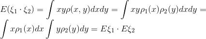
- The mean values of the errors are zero:
.
- The very law of the distribution of random variables may not be known to us, but their variances are known.
and
. Note that dispersions are independent of
- It is assumed that all random errors are independent of each other: what error will be at the moment of time
.
It is worth noting that the filtering task is not a smoothing task. We do not strive to smooth the data from the sensor, we strive to get the closest value to the real coordinate
Kalman algorithm
We will reason by induction. Imagine that on
therefore, without yet getting the value from the sensor, we can assume that in step
The idea of Kalman is that in order to get the best approximation to the true coordinate
Coefficient
We must choose the Kalman coefficient
In general, to find the exact value of the Kalman coefficient
Use equations (1) (those that are on a blue background in a frame) to rewrite the expression for the error:
Evidence
Now it's time to discuss what the expression means to minimize the error? After all, the error, as we see, is in itself a random variable and each time takes on different values. In fact, there is no unambiguous approach to determining what the error means is minimal. Just as in the case of the variance of a random variable, when we tried to estimate the characteristic width of its spread, so here we will choose the most simple criterion for calculations. We will minimize the average of the squared error:
Let's write the last expression:
key to proof
From the fact that all random variables in the expression for  , independent and average values of sensor errors and models are zero:
  , it follows that all "cross" members are equal to zero:
 .
.
Plus, the formulas for dispersions look much simpler: and
and  (because )
Plus, the formulas for dispersions look much simpler:
This expression takes the minimum value when (we equate the derivative with zero)
Here we are already writing the expression for the Kalman coefficient with the step index
Substitute the expression for the root-mean-square error
Our problem is solved. We obtained an iterative formula for calculating the Kalman coefficient.
All formulas in one place
Example
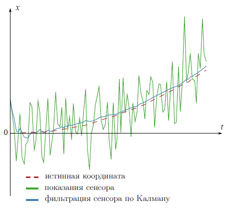
The advertising picture at the beginning of the article filtered data from a fictional GPS sensor mounted on a fictional car that travels evenly accelerated with known fictional acceleration
Look again at the result of filtering.
Code on matlabe
clear all; N=100 % number of samples a=0.1 % acceleration sigmaPsi=1 sigmaEta=50; k=1:N x=k x(1)=0 z(1)=x(1)+normrnd(0,sigmaEta); for t=1:(N-1) x(t+1)=x(t)+a*t+normrnd(0,sigmaPsi); z(t+1)=x(t+1)+normrnd(0,sigmaEta); end; %kalman filter xOpt(1)=z(1); eOpt(1)=sigmaEta; % eOpt(t) is a square root of the error dispersion (variance). It's not a random variable. for t=1:(N-1) eOpt(t+1)=sqrt((sigmaEta^2)*(eOpt(t)^2+sigmaPsi^2)/(sigmaEta^2+eOpt(t)^2+sigmaPsi^2)) K(t+1)=(eOpt(t+1))^2/sigmaEta^2 xOpt(t+1)=(xOpt(t)+a*t)*(1-K(t+1))+K(t+1)*z(t+1) end; plot(k,xOpt,k,z,k,x) Analysis
If you follow up with an iteration step

In the following example, we will discuss how this will help to significantly ease our lives.
Second example
In practice, it often happens that we do not know anything at all about the physical model of what we filter. For example, you wanted to filter readings from your favorite accelerometer. You also do not know in advance by what law you intend to turn the accelerometer. The maximum information you can use is the variance of the sensor error.
But, frankly, such a system does not at all satisfy the conditions that we imposed on a random variable.
But you can go the other way, a much simpler way. As we saw above, the Kalman coefficient
The following graph shows data filtered in two different ways from a fictional sensor. Provided that we know nothing about the physics of the phenomenon. The first method is honest, with all the formulas from Kalman's theory. And the second is simplified, without formulas.

As we see, the methods are almost the same. A small difference is observed only at the beginning, when the Kalman coefficient has not yet stabilized.
Discussion
As we have seen, the main idea of the Kalman filter is to find the coefficient
on average, the least would be different from the real value of the coordinate
Therefore, the Kalman filter is called a linear filter.
It is possible to prove that of all linear filters, the Kalman filter is the best. Best in the sense that the mean square error of the filter is minimal.
Multidimensional case
The whole theory of the Kalman filter can be generalized to the multidimensional case. The formulas there look a little worse, but the very idea of their derivation is the same as in the one-dimensional case. In this beautiful article you can see them: http://habrahabr.ru/post/140274/ .
And in this wonderful video, an example of how to use them is analyzed.
Literature
You can download the original Kalman article here: http://www.cs.unc.edu/~welch/kalman/media/pdf/Kalman1960.pdf .
This post can be read in English http://david.wf/kalmanfilter
Source: https://habr.com/ru/post/166693/
All Articles