Dynamic visualization of geocoded data (Twitter) using R

"New Year is sweeping the country"

I am an ardent fan of geosocial services. They allow you to visually see the physical realization of social space. This is what Bourdieu wrote about, but what was available to him only in the form of a mental construct. Foursquare is generally my unrequited love. But about this sometime next time, and today we will talk about Twitter.
Shortly before the end of the previous 2012 year, I wanted to see what the “wave” of the New Year greetings tweets looks like. See how it goes through time zones. No sooner said than done. Used tools: R, Python and ffmpeg.

Data collection

While the spouse took up the holiday preparations and didn’t remember about me, using python and tweetstream we did the primitive tweet-stream statuses / filter parser.

import tweetstream stream = tweetstream.FilterStream('TWITTER_LOGIN', 'TWITTER_PASSWORD', track = keywords_list) for tweet in stream: if tweet['coordinates']: #      date-time  # ( API Twitter     ) try: timestamp = datetime.datetime.strptime(tweet['created_at'], '%Y-%m-%d %H:%M:%S') except ValueError: timestamp = datetime.datetime.strptime(tweet['created_at'][4:-10]+tweet['created_at'][-4:], '%b %d %H:%M:%S %Y') #  4  - ""    timestamp += datetime.timedelta(hours=4) #       timestamp = datetime.datetime.strftime(timestamp, '%Y-%m-%d %H:%M:%S') #     cursor.execute('INSERT INTO tweets(link, latitude, longitude, date) VALUES ("http://www.twitter.com/{0}/status/{1}", "{2}", "{3}", "{4}")'.format( tweet['user']['screen_name'], tweet['id'], str(tweet['coordinates']['coordinates'][0]), str(tweet['coordinates']['coordinates'][1]), str(tweet['created_at']) )) db.commit() 

keywords_list - A list of keywords, hash tags and phrases related to Happy New Year greetings. Do not forget that this API call does not take into account the morphology, so you should try to enter as many relevant word forms as possible into the keywords. My list is:

• #happy New Year,
• #New Year2013,
• #NG2013,
• # Oncoming2013,
• #New Year,
• #Happy New Year,
• # NEW YEAR,
• happy New Year,
• holiday greetings,
• new 2013
• with the year of the snake,
• Happy New Year of the Snake
• New Year,
• new year.

Everything, the spouse paid attention to excess hands, so we start the parser and we hasten to the rescue. Finally, we contribute to the “increase in entropy”:

Review of the data

Night from Friday to Monday, the first days of the new year flew by unnoticed. The holiday has passed, the parser can be turned off and look at the "catch". Total recruited ~ 10 thousand tweets. Geotags on Twitter are not popular. For mobility, I dumped a dump into a .csv table like "link - latitude - longitude - timestamp". Ship the table in R:

 twits <- read.csv2('ny_tweets.csv', header=F) colnames(twits) <- c('Link', 'Longitude', 'Latitude', 'Timestamp') twits$Timestamp <- strptime(twits$Timestamp, format='%Y-%m-%d %H:%M:%S') twits$Latitude <- round(as.numeric(as.character(twits$Latitude)), digits=1) twits$Longitude <- round(as.numeric(as.character(twits$Longitude)), digits=1) twits$Longitude <- sapply(twits$Longitude, function(x){ if(x < (-169)){ x<-360+x } else {x} }) 

We translate timestamps into the appropriate format, round latitude and longitude - we will watch Twitter activity on the grid in one tenth of a degree. The last longitude transformation is necessary for further visualization in order not to lose messages from Chukotka.
Now we load ggplot2 and see the distribution in time:

 library('ggplot2') p <- ggplot() p <- p + geom_histogram(aes(x=twits$Timestamp, fill = ..count..), binwidth = 3600) p <- p + ylab('') + xlab(' ( )') p <- p + theme(legend.position = 'none') p <- p + ggtitle(expression(' "" ')) p 

Everything looks approximately as expected, which pleasantly pleases. We can continue.

Map drawing

Ggplot2 offers a rich set of tools for quickly building informative and cute graphs. Full documentation with examples: ggplot docs .
To draw a map, we will use the geom_polygon function, which allows us to draw polygons according to given coordinates. The contours of the countries will be taken from the maps library. The drawing variant described in the article “How to draw good looking maps in R” was taken as a basis. We slightly modify the described version, adjusting it to our own needs and “ideas about beauty”:

 #    # countries -    ,    library('maps') full_map <- map_data('world') table(full_map$region) need.map <- subset(full_map, region %in% countries & long>-25 & long<190 & lat>25) #   p <- ggplot() p <- p + geom_polygon(aes(x=need.map$long, y=need.map$lat, group = need.map$group), colour='white', fill='grey20', alpha=.5) #  ""     " " # cities -  dataframe  "  -  - " p <- p + geom_point(aes(cities$Long, cities$Lat), colour='skyblue', size=1.5) #    , ,     ,   p <- p + theme(axis.line=element_blank(),axis.text.x=element_blank(), axis.text.y=element_blank(),axis.ticks=element_blank(), axis.title.x=element_blank(), axis.title.y=element_blank(), legend.position = 'none', text=element_text(family='mono', size=20, face='bold', colour='dodgerblue3') ) p <- p + scale_x_continuous(limits = c(-15, 190)) p <- p + scale_y_continuous(limits = c(30, 82)) p <- p + ggtitle(expression('#HappyNewYear in Russian Twitter - 2013')) 

I want to somehow revive the picture and add information. Let's put a clock in the frame. Here is an interesting option with a clock: Create an animated clock in ggplot2 (and ffmpeg) . But it uses a polar coordinate system that does not suit us, because will require extra gestures in the form of creating sub-graphics. You have to do your "bike". We take the function to calculate the coordinates of the circle in the center and diameter (peeped here ):

 draw.circle <- function(center,diameter=1, npoints = 100){ r = diameter / 2 tt <- seq(0,2*pi,length.out = npoints) xx <- center[1] + r * cos(tt) yy <- center[2] + r * sin(tt) * roundcoef return(data.frame(x = xx, y = yy)) } 

Now we count the points for three circles: a white background backdrop, a gray “upper” background and 12 points on the circle for the hour serifs:

 curtime <- c(as.numeric(format(frame.time, '%H')), as.numeric(format(frame.time, '%M'))) clock.center <- c(180, 35) circdat <- draw.circle(clock.center, diameter=20) circdat2 <- draw.circle(clock.center, diameter=19.7) circdat3 <- draw.circle(clock.center, diameter=18, npoints=13) 

We consider the position of the arrows:

 arrow.r = c(5.5,8.8) #   if(curtime[1]>=12){curtime[1]=curtime[1]-12} hourval <- pi*(.5 - (curtime[1]+(curtime[2]/60))/6) minval <- pi*(.5 - curtime[2]/30) hour.x <- clock.center[1] + arrow.r[1] * cos(hourval) hour.y <- clock.center[2] + arrow.r[1] * sin(hourval) minute.x <- clock.center[1] + arrow.r[2] * cos(minval) minute.y <- clock.center[2] + arrow.r[2] * sin(minval) 

Draw a clock (functions geom_polygon, geom_segment, geom_point):

 #  :     p <- p + geom_polygon(aes(x=circdat$x,y=circdat$y), colour='grey100', fill='grey100', alpha = .5) p <- p + geom_polygon(aes(x=circdat2$x,y=circdat2$y), colour='grey80', fill='grey80', alpha = .5) p <- p + geom_point(aes(circdat3$x, circdat3$y), colour='skyblue') #  , , ""   p <- p + geom_segment(aes(x=clock.center[1], y=clock.center[2], xend=hour.x, yend=hour.y), size=3, colour='dodgerblue3') p <- p + geom_segment(aes(x=clock.center[1], y=clock.center[2], xend=minute.x, yend=minute.y), size=1.5, colour='dodgerblue4') p <- p + geom_point(aes(clock.center[1], clock.center[2]), colour='blue4') 

This is what happened (on the map there are also test data on “activity”, but only in Moscow and the surrounding area):

')

Draw frames

Baseline - a table with the coordinates and time of publication of the tweet. At the exit, we want to get a set of frames. Let's do this: we will set the time of the 1st frame, the time of the last frame and the time difference between adjacent frames in the settings. The total number of frames will be calculated in R. Next is the cycle from 1 to the last frame. In each frame, the “current” time will be calculated. Next - from the source table we will select tweets that fall in the required time interval (30 minutes before the “current” frame time - the “current” frame time).

 start.date <- '2012-12-31 00:00:00' finish.date <- '2013-01-01 12:00:00' seconds.in.frame <- 30 start.date <- strptime(start.date, format='%Y-%m-%d %H:%M:%S') finish.date <- strptime(finish.date, format='%Y-%m-%d %H:%M:%S') frames <- as.numeric(difftime(finish.date, start.date, units='secs'))/seconds.in.frame for(i in 1:frames){ frame.time <- start.date + i*seconds.in.frame frame.twits <- subset(twits, Timestamp <= frame.time & Timestamp > frame.time - ma.period) ... 

Next, we make the “latitude - longitude” contingency table (recall that the values ​​of latitude and longitude were previously converted from continuous to discrete by rounding to one-tenth). And we “expand” the contingency table in the dataframe of 3 columns: latitude, longitude, frequency (number of tweets at a given point). We remove the lines in which the frequency is zero or the coordinates are outside the established limits.

  ... frame.twits <- melt(table(frame.twits$Latitude, frame.twits$Longitude)) colnames(frame.twits) <- c('Lat', 'Long', 'Volume') frame.twits$Lat <- as.numeric(as.character(frame.twits$Lat)) frame.twits$Long <- as.numeric(as.character(frame.twits$Long)) frame.twits <- frame.twits[frame.twits$Volume>0 & frame.twits$Long>=-25 & frame.twits$Long<=190 & frame.twits$Lat>=25 & frame.twits$Lat<=85,] ... 

The transformation of latitude and longitude into numerical variables is necessary because after the “folding-unfolding” of the data, they are converted into categorical (factor in the terminology of R).
It remains to calculate the colors of the points. To do this, the maximum possible volume of tweets at one point for the whole future “movie” is calculated in the preliminary cycle. It takes the maximum ( max.color ), and colors for all other points are calculated relative to it (logarithm - to “align” the scale):

  ... frame.colors <- round(1 + (8*log(frame.twits$Volume)/max.color), digits=0) ... 

Now you can draw points (if any):

  ... if(nrow(frame.twits)>0){ p <- p + geom_point(aes(frame.twits$Long,frame.twits$Lat, size=frame.twits$Volume * 5), colour=twits.colors[frame.colors], alpha = .75) } ... 

It seems to be all, you can save the image and close the loop, but for the next "animate the picture" I decided to add some real messages to the frame. To do this, I randomly selected dozens of tweets from the general array, collected message texts for them and created another dataframe - publication time, tweet text, “lifetime”, “appearance time”, “extinction time”, color, coordinates, size and transparency . The lifetime, coordinates, color and size are generated when the script is initialized with random deviations from the “optimal” values:

 twit.texts$x <- rnorm(nrow(twit.texts), mean = 100, sd = 30) twit.texts$y <- rnorm(nrow(twit.texts), mean = 56, sd = 15) twit.texts$size <- rnorm(nrow(twit.texts), mean = 10, sd = 2) 

Output to the frame is controlled using transparency: if the “current” frame time does not fit into the “lifetime” of a tweet, its “opacity” is zero. If the current tweet "exists" - its opacity is calculated depending on the proximity to the center of the life period. It turns out that the tweet "appears" and smoothly disappears. In code, it looks like this:

  ... twit.texts$opacity <- as.numeric(by(twit.texts, 1:nrow(twit.texts), function(row){ if(frame.time < row$t.start | frame.time > row$t.end){ row$opacity <- 0 } else { row$opacity <- 0.7 * (1 - (abs(as.numeric(difftime(row$Timestamp, frame.time, unit='sec'))) / (row$t.delta * seconds.in.frame / 2))) } })) p <- p + geom_text(aes(x=twit.texts$x, y=twit.texts$y, label=iconv(twit.texts$Text,to='UTF-8')), colour=twit.texts$color, size=twit.texts$size, alpha = twit.texts$opacity) ... 

The output is organized using geom_text.
Now that's it. You can save the frame and close the loop.

  ... f.name <- as.character(i) repeat{ if(nchar(f.name) < nchar(as.character(frames))){ f.name <- paste('0', f.name, sep='') } else { break }} ggsave(p, file=paste('frames/img', f.name, '.png', sep=''), width=6.4, height=3.6, scale = 3, dpi=100) } 

The length of f.name "zeros" is adjusted so that all names "fit" under one mask by the number of characters.

We collect video

To build the final video, ffmpeg was used:
ffmpeg -f image2 -i img%04d.png -q:v 0 -vcodec mpeg4 -r 24 happynewyear.mp4
However, not all so simple. The video is not fully assembled - the .png files received from ggplot2 have different color depths. Perhaps this problem could be solved in some more correct way, but I used the Python Imaging Library :

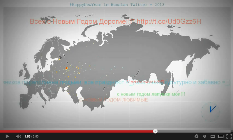
 import os from PIL import Image path = u'/path/to/frames/' dirList=os.listdir(path) for filename in dirList: if filename[-3:] == 'png': im = Image.open(path + filename).convert('RGB') im.save(path + filename) 

Now all frames are collected in one video. The video is ready, you can upload to YouTube. Add a couple of YouTube-effects (because if the gun hangs on the wall, you need to shoot from time to time).
The final:

In this text I have described not all parts of the R-script, but some of the quotes from the code are arranged according to the principle of the problem being solved, and not according to the logic of the work. Therefore, in the application I post a link to the full code with a small number of comments: pastebin.com

Possible options for development

1. Add date because The 12-hour dial is not too informative when you need to visualize the time interval of several days.
2. Add a strip with a histogram or something like a probability density graph for the total amount of data at each time point.

Questions to the community

1. Is there a library for R comparable in simplicity to maps, but with more relevant information on modern geopolitics? Without USSR, Yugoslavia and Czechoslovakia?
2. How can you try to optimize the calculation of the colors of the palette of dots so as not to “run” the entire cycle “idle” beforehand?
3. Is it possible to "overcome" ggplot2 or ffmpeg, so that additional frame color conversion is not required (exclude PIL from the process)?
4. And in general - I will listen to other indications of my own humanitarian curvature and optimization possibilities.

Thank!

useful links

1. How to draw good looking maps in R - using maps and ggplot2 to draw maps;
2. Create an animated clock in R with ggplot2 (and ffmpeg) - animated analog clock on R;
3. Simple data mining and plotting data on a map with ggplot2 - using OSM maps in R.