Pre-training of the neural network using a limited Boltzmann machine
Hey. As planned in the past post about limited Boltzmann machines, this will consider the use of RBM for the pre-training of an ordinary multilayered network of direct distribution . Such a network is usually trained in the back-propagation error algorithm , which depends on many parameters, and so far there is no exact algorithm for choosing these training parameters, as well as the optimal network architecture. Many heuristics have been developed to reduce the search space, as well as methods for assessing the quality of selected parameters (for example, cross-validation ). Moreover, it turns out that the back-propagation algorithm itself is not so good. Although Rumelhart, Hinton, and Williams showed convergence of the back-propagation algorithm (here is even more mathematical proof of convergence ), but there is a small nuance: the algorithm converges with infinitesimally small changes in weights (that is, with the learning rate tending to zero). And even that is not all. Typically, this algorithm teaches small networks with one or two hidden layers due to the fact that the effect of training does not reach the distant layers. Next, we will talk more about why it does not reach , and apply the weights initialization technique with the help of a trained RBM, which was developed by Jeffrey Hinton .
To begin, let's take a look at the graphs that look the same.
')

They depict the dependence of the average weight change in the layer (y-axis) on the epochs of training (the x-axis). A network of the following structure was studied: six layers, 5 hidden 100 neurons and an output of 26 neurons (the number of classes, or letters in the English alphabet).
As you can see, the dynamics are basically the same, but the minimum average change in weights in the output layer is of the same order as the maximum - in the third hidden layer, and in the far layers - even less. In this case, we observe a gradient decay, and the opposite picture is called “explosive growth of the gradient” (in English literature this is called “vanishing and exploding gradients”), to see this effect, it is enough to initialize the weights with large values. In order to understand mathematics, I advise you to refer, for example, to these articles:
And we will now try to figure out on the fingers the causes of this phenomenon, based on how it was presented in the course on neural networks on the cursor . So, what is the direct passage of a signal through a neural network? On each layer, a linear combination of the input signal of the layer and the weights of each neuron is calculated, the result is a scalar in each neuron, and then the value of the activation function is calculated. As a rule, the activation function, in addition to the nonlinearity we need, helps to limit the output values of neurons, but we consider only the activation function of a general form. Thus, the output is a vector, each component of which is within the previously known limits.

Now look at the back pass. Gradients on the output layer are easily calculated and significant changes in the weights of the neurons of the output layer are obtained. For any hidden layer, recall the formula for calculating the gradient:
If we replace the expression dE / dz, where k is involved, delta,

we will see that the reverse passage is very similar to the straight line, but it is completely linear, with all the ensuing consequences. A delta is called a local gradient / neuron error. During the reverse passage of the delta can be interpreted as exits (in the other direction) of the corresponding neurons. The value of the weight gradient of the neuron of the deeper layer is proportional to the value of the derivative of the activation function at the point obtained in the forward passage. Recall the geometric definition of the derivative at a point:

x0 is calculated and fixed during the forward pass. These are the red lines in the picture above. And it turns out that the linear combination of weights and local gradients of neurons is multiplied by this value, which is the tangent of the tangent angle at x0, and the range of tangent values is known to be in the range from minus infinity to plus infinity.
The reverse pass for one neuron of the hidden layer is as follows:

What we have in the end:
As a rule, shallow nets do not suffer from this due to the small number of layers, since the effect does not have time to accumulate during the backward pass (we will consider an example of accumulation in the next section).
If sigmoid is used as an activation function
with a derivative of the following form:

then for α = 1 we can easily verify that the maximum value reached by the derivative is 0.25 at the point x = 0.5, and the minimum value is 0 at the points x = 0 and x = 1 (in the interval from 0 to 1, the range of values is logistic functions):

Consequently, for networks with a logistic activation function, explosive growth and attenuation largely depend on the value of the weights, although there is a permanent attenuation due to the fact that at best the tangent of the tangent angle is only 0.25, and these values, as we will see in next section, from layer to layer are multiplied together:
To illustrate the above, consider an example.

Given a simple network that minimizes the square of the Euclidean distance, with the logistic activation function, we find the gradients of weights with the input image x = 1 and the target t = 0.5.
After the direct passage, we obtain the output values of each neuron: 0.731058578630005, 0.188143725087062, 0.407022630083087, 0.307029145835665, 0.576159944190332. Denote them by y1, ..., y5.
As you can see, the gradient decays. In the course of the calculation, it is noticeable that the accumulation occurs due to the multiplication of the weights and the values of the derivatives of the current layer and all subsequent ones. Although the initial values are far from small, compared to how the weights are initialized in practice, these values are not enough to suppress the permanent attenuation from the tangents of the tangent angle.
Before talking about the method proposed by Jeffrey Hinton , it is worth noting immediately that today there is no formal mathematical proof that preliminary fine-tuning of the scales guarantees an improvement in the quality of the network. So, Hinton suggested using limited Boltzmann machines to pre-tune the scales. As in the post about RBM, we will now talk only about binary input images, although this model extends to input images consisting of real numbers .
Suppose we have a network of direct distribution of the following structure:

Such a network was called Deep Belief Networks .
As I said, the effectiveness of this method is not proven, as well as the effectiveness of any fine initialization, but the fact remains that it works. The explanation for this effect can be given as follows: when learning the very first RBM, we create a model that generates some hidden signs from visible states, that is, we immediately put the weights at some minimum necessary to calculate these signs; with each subsequent layer, signs of signs are calculated, and weights are always placed in a state sufficient to calculate these hierarchical signs; when it comes to training with a teacher, in fact, only 2-3 layers of the output will be effectively trained, based on those hyper-signs that were calculated earlier, and those, in turn, will change slightly to suit the task. Hence, we can assume that it is not necessary to initialize all layers in this way, and the output, and possibly 1-2 hidden ones, can be initialized usually, for example, by selecting numbers from the normal distribution with center 0 and variance 0.01.
Experiments play an important role in this post, so you should immediately make a reservation about the sets used for training and model testing. I generated several small and easy to summarize sets so that no more than 30 minutes were spent on learning networks.
In all experiments, learning will stop when the following condition is met (both learning of direct distribution networks and Boltzmann machines). We introduce the notation:
So, the learning process will be interrupted if the following condition is met:

those. if the increase in cross-validation error is greater than a certain percentage of the minimum error, then stop.
In direct propagation networks, the output layer will be the softmax layer , and the entire network is trained to minimize cross-entropy , respectively, the error value is calculated in the same way. And the limited Boltzmann machines will use the Hamming distance between the binary input and the binary recovered manner as a measure of error.
To begin with, let's see what result will give us a network with one hidden layer of 100 neurons, i.e. its structure will be
Learning options:

The result on the test set, the training took about 35 seconds:
Error: 1.39354424678178
Wins: 231 of 312, 74.03%
If the pre-trained network shows the result below this, it will be very sad -). We will pre-train a network of 5 layers of the following structure:
Learning options:

The results on the test set are insignificant, about 3 hits from 312. Training took 4300 seconds, which is almost an hour and twenty (training was interrupted for the 2000 era, although it could have continued further). For 2000 epochs, an error value of 3.25710954400557 was reached, while in the previous test already at the second epoch it was 3.2363407570674, and at the last one 0.114535596947578.
And now let's train RBMs for each consecutive pair. For starters, it will be

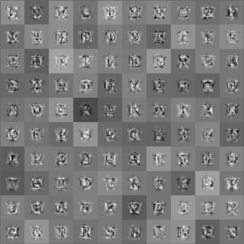
Training took 1274 seconds. The first pair is easy to visualize, as was done in the previous post. The following patterns are obtained:

Increase a little:
Then we train the second pair of

We train the third pair

We don’t touch the weights of the output layer and the first hidden layer and initialize it with random values from the normal distribution with center 0 and variance 0.01. Now we put all layers into one direct distribution network and train with the following parameters:

The result on the test set, while learning took only 17 epochs or 36 seconds:
Error: 1.40156176438071
Wins: 267 of 312, 85.57%
The increase in quality was almost 11% compared to the network with one hidden layer. I, frankly, expected more, but here it is already a matter of data complexity . As experiments have shown and confirmed the read articles, the more complex and large data we have, the greater the increase in quality will be obtained.
Pre-training is obviously an effective way -) Perhaps some mathematical genius will prove its effectiveness in theory, and not only in practice, as it is now.
Suppose there is a task to recognize captcha. We have downloaded 100,000 images, only 10,000 of them are manually recognized. We would like to train the neural network, but we feel sorry not to use the remaining 90,000 thousand images. This is where RBM comes to the rescue. Using an array of 100,000 images, we train a deep belief network, and then on a set of 10,000 hand-recognized images, we train a deep network. Profit!
Thanks to the user OTHbIHE for help in editing the article!
Attenuation and explosive growth of weight changes
To begin, let's take a look at the graphs that look the same.
')
They depict the dependence of the average weight change in the layer (y-axis) on the epochs of training (the x-axis). A network of the following structure was studied: six layers, 5 hidden 100 neurons and an output of 26 neurons (the number of classes, or letters in the English alphabet).
| input dimension = 841 | layer -5 | layer -4 | layer -3 | layer -2 | layer -1 | output |
| 100 neurons | 100 neurons | 100 neurons | 100 neurons | 100 neurons | 26 neurons |
As you can see, the dynamics are basically the same, but the minimum average change in weights in the output layer is of the same order as the maximum - in the third hidden layer, and in the far layers - even less. In this case, we observe a gradient decay, and the opposite picture is called “explosive growth of the gradient” (in English literature this is called “vanishing and exploding gradients”), to see this effect, it is enough to initialize the weights with large values. In order to understand mathematics, I advise you to refer, for example, to these articles:
- Understanding the training network of deep feedforward neural networks
- Understanding the exploding gradient problem
And we will now try to figure out on the fingers the causes of this phenomenon, based on how it was presented in the course on neural networks on the cursor . So, what is the direct passage of a signal through a neural network? On each layer, a linear combination of the input signal of the layer and the weights of each neuron is calculated, the result is a scalar in each neuron, and then the value of the activation function is calculated. As a rule, the activation function, in addition to the nonlinearity we need, helps to limit the output values of neurons, but we consider only the activation function of a general form. Thus, the output is a vector, each component of which is within the previously known limits.
Now look at the back pass. Gradients on the output layer are easily calculated and significant changes in the weights of the neurons of the output layer are obtained. For any hidden layer, recall the formula for calculating the gradient:
If we replace the expression dE / dz, where k is involved, delta,
we will see that the reverse passage is very similar to the straight line, but it is completely linear, with all the ensuing consequences. A delta is called a local gradient / neuron error. During the reverse passage of the delta can be interpreted as exits (in the other direction) of the corresponding neurons. The value of the weight gradient of the neuron of the deeper layer is proportional to the value of the derivative of the activation function at the point obtained in the forward passage. Recall the geometric definition of the derivative at a point:
x0 is calculated and fixed during the forward pass. These are the red lines in the picture above. And it turns out that the linear combination of weights and local gradients of neurons is multiplied by this value, which is the tangent of the tangent angle at x0, and the range of tangent values is known to be in the range from minus infinity to plus infinity.
The reverse pass for one neuron of the hidden layer is as follows:
What we have in the end:
- explosive growth can occur if the weights are too large, or the value of the derivative at the point is too large
- damping occurs if the value of the weights or the derivative at the point is very small
As a rule, shallow nets do not suffer from this due to the small number of layers, since the effect does not have time to accumulate during the backward pass (we will consider an example of accumulation in the next section).
If sigmoid is used as an activation function
with a derivative of the following form:
then for α = 1 we can easily verify that the maximum value reached by the derivative is 0.25 at the point x = 0.5, and the minimum value is 0 at the points x = 0 and x = 1 (in the interval from 0 to 1, the range of values is logistic functions):
Consequently, for networks with a logistic activation function, explosive growth and attenuation largely depend on the value of the weights, although there is a permanent attenuation due to the fact that at best the tangent of the tangent angle is only 0.25, and these values, as we will see in next section, from layer to layer are multiplied together:
- for very small weights, attenuation occurs
- with sufficiently large scales - growth
Simple example
To illustrate the above, consider an example.
Given a simple network that minimizes the square of the Euclidean distance, with the logistic activation function, we find the gradients of weights with the input image x = 1 and the target t = 0.5.
After the direct passage, we obtain the output values of each neuron: 0.731058578630005, 0.188143725087062, 0.407022630083087, 0.307029145835665, 0.576159944190332. Denote them by y1, ..., y5.


As you can see, the gradient decays. In the course of the calculation, it is noticeable that the accumulation occurs due to the multiplication of the weights and the values of the derivatives of the current layer and all subsequent ones. Although the initial values are far from small, compared to how the weights are initialized in practice, these values are not enough to suppress the permanent attenuation from the tangents of the tangent angle.
Pretraining
Before talking about the method proposed by Jeffrey Hinton , it is worth noting immediately that today there is no formal mathematical proof that preliminary fine-tuning of the scales guarantees an improvement in the quality of the network. So, Hinton suggested using limited Boltzmann machines to pre-tune the scales. As in the post about RBM, we will now talk only about binary input images, although this model extends to input images consisting of real numbers .
Suppose we have a network of direct distribution of the following structure:
x1 -> x2 -> ... -> xn , where each xi is the number of neurons in the layer, xn is the output layer. Let x0 be the dimension of the input image, which is fed to the input, i.e. on layer x1. We also have a dataset for training, data (we denote D0) are pairs of the “input, expected output” type, and we want to train the network using the back-propagation error algorithm . But before that, we can accomplish a fine initialization of the scales, for this:- We consistently train one RBM for each consecutive pair of layers, including the dummy layer x0, and we end up with exactly n pieces of RBM. To begin with, the first pair
x0 <-> x1is taken, she is trained on a set of input images from D0 (this is training without a teacher). Then, for each input image from D0, the derivation of the probabilities of the hidden layer and sampling is made, we get a set of binary vectors D1. Then, using D1, the pairx1 <-> x2trained. And so on tox{n-1} <-> xn. - We disassemble each RBM, and take the second layers with their own weights.
- From the selected second layers of each RBM we compose the initial network
x1 -> x2 -> ... -> xn.
Such a network was called Deep Belief Networks .
As I said, the effectiveness of this method is not proven, as well as the effectiveness of any fine initialization, but the fact remains that it works. The explanation for this effect can be given as follows: when learning the very first RBM, we create a model that generates some hidden signs from visible states, that is, we immediately put the weights at some minimum necessary to calculate these signs; with each subsequent layer, signs of signs are calculated, and weights are always placed in a state sufficient to calculate these hierarchical signs; when it comes to training with a teacher, in fact, only 2-3 layers of the output will be effectively trained, based on those hyper-signs that were calculated earlier, and those, in turn, will change slightly to suit the task. Hence, we can assume that it is not necessary to initialize all layers in this way, and the output, and possibly 1-2 hidden ones, can be initialized usually, for example, by selecting numbers from the normal distribution with center 0 and variance 0.01.
Initial data
Experiments play an important role in this post, so you should immediately make a reservation about the sets used for training and model testing. I generated several small and easy to summarize sets so that no more than 30 minutes were spent on learning networks.
- The training set consists of images of large print letters of the English alphabet of three fonts ( Arial , Courier and Times as representatives of different breeds ) of 29 by 29 pixels in size, and their images with some random noises.
- The cross-validation set consists of the same set of fonts, plus Tahoma and a bit more noise
- The test set consists of the same data set as the cross-validation, differs only in the randomness factor in the generation of noise
In all experiments, learning will stop when the following condition is met (both learning of direct distribution networks and Boltzmann machines). We introduce the notation:
 - This is a cross-validation error of the current era.
 - this is a cross-validation error in the past era
 - this is the minimum cross-validation error achieved from the beginning of the learning process to the current era
- k - stop parameter with an increase in the cross-validation error, from the interval (0, 1)
So, the learning process will be interrupted if the following condition is met:
those. if the increase in cross-validation error is greater than a certain percentage of the minimum error, then stop.
In direct propagation networks, the output layer will be the softmax layer , and the entire network is trained to minimize cross-entropy , respectively, the error value is calculated in the same way. And the limited Boltzmann machines will use the Hamming distance between the binary input and the binary recovered manner as a measure of error.
Experiments
To begin with, let's see what result will give us a network with one hidden layer of 100 neurons, i.e. its structure will be
100 -> 26 . We illustrate each learning process with a schedule with a learning error and cross-validation.Learning options:
- LearningRate = 0.001
- BatchSize = full batch
- RegularizationFactor = 0
- Momentum = 0.9
- NeuronLocalGainLimit: Limit = [0.1, 10]; Bonus = 0.05; Penalty = 0.95
- CrossValidationStopFactor is 0.05
The result on the test set, the training took about 35 seconds:
Error: 1.39354424678178
Wins: 231 of 312, 74.03%
If the pre-trained network shows the result below this, it will be very sad -). We will pre-train a network of 5 layers of the following structure:
100 -> 300 -> 100 -> 50 -> 26 . But first, let's see how the learning process and the result look like if we train such a network without pre-training.Learning options:
- LearningRate = 0.001
- BatchSize = full batch
- RegularizationFactor = 0.1
- MaxEpoches = 2000
- MinError = 0.1
- Momentum = 0
- NeuronLocalGainLimit: not setted
- CrossValidationStopFactor is 0.001
The results on the test set are insignificant, about 3 hits from 312. Training took 4300 seconds, which is almost an hour and twenty (training was interrupted for the 2000 era, although it could have continued further). For 2000 epochs, an error value of 3.25710954400557 was reached, while in the previous test already at the second epoch it was 3.2363407570674, and at the last one 0.114535596947578.
And now let's train RBMs for each consecutive pair. For starters, it will be
841 <-> 100 with the following parameters:- LearningRate = 0.001
- BatchSize = 10
- Momentum = 0.9
- NeuronLocalGainLimit: Limit = [0.001, 1000]; Bonus = 0.0005; Penalty = 0.9995
- GibbsSamplingChainLength = 35
- UseBiases = True
- CrossValidationStopFactor is 0.5
- MinErrorChange = 0.0000001
Training took 1274 seconds. The first pair is easy to visualize, as was done in the previous post. The following patterns are obtained:
Increase a little:
Then we train the second pair of
100 <-> 300 , it took 2095 seconds:- LearningRate = 0.001
- BatchSize = 10
- Momentum = 0.9
- NeuronLocalGainLimit: Limit = [0.001, 1000]; Bonus = 0.0005; Penalty = 0.9995
- GibbsSamplingChainLength = 35
- UseBiases = True
- CrossValidationStopFactor is 0.1
We train the third pair
300 <-> 100 , took 1300 seconds:- LearningRate = 0.001
- BatchSize = 10
- Momentum = 0.9
- NeuronLocalGainLimit: Limit = [0.001, 1000]; Bonus = 0.0005; Penalty = 0.9995
- GibbsSamplingChainLength = 35
- UseBiases = True
- CrossValidationStopFactor is 0.1
We don’t touch the weights of the output layer and the first hidden layer and initialize it with random values from the normal distribution with center 0 and variance 0.01. Now we put all layers into one direct distribution network and train with the following parameters:
- LearningRate = 0.001
- BatchSize = full batch
- RegularizationFactor = 0
- Momentum = 0.9
- NeuronLocalGainLimit: Limit = [0.01, 100]; Bonus = 0.005; Penalty = 0.995
- CrossValidationStopFactor is 0.01
The result on the test set, while learning took only 17 epochs or 36 seconds:
Error: 1.40156176438071
Wins: 267 of 312, 85.57%
The increase in quality was almost 11% compared to the network with one hidden layer. I, frankly, expected more, but here it is already a matter of data complexity . As experiments have shown and confirmed the read articles, the more complex and large data we have, the greater the increase in quality will be obtained.
Conclusion
Pre-training is obviously an effective way -) Perhaps some mathematical genius will prove its effectiveness in theory, and not only in practice, as it is now.
Suppose there is a task to recognize captcha. We have downloaded 100,000 images, only 10,000 of them are manually recognized. We would like to train the neural network, but we feel sorry not to use the remaining 90,000 thousand images. This is where RBM comes to the rescue. Using an array of 100,000 images, we train a deep belief network, and then on a set of 10,000 hand-recognized images, we train a deep network. Profit!
Links
- Learning Internal Representations by Error Propagation
- Understanding the training network of deep feedforward neural networks
- Understanding the exploding gradient problem
- Deep Boltzmann Machines
- A Practical Guide to Training Restricted Boltzmann Machines
- Deep Belief Networks
Thanks to the user OTHbIHE for help in editing the article!
Source: https://habr.com/ru/post/163819/
All Articles