What the mess looks like or whether the fascists have homing missiles

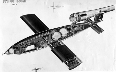June 13, 1944, a week after the Allied invasion of Normandy, a loud humming sound boomed in the sky of London battered by battles. The sound source was the newly developed German cannon of war: the V-1 aerial bomb. A predecessor of cruise missiles, the V-1 was a self-propelled bomb controlled by gyros, powered by a simple pulsating jet engine that absorbed air and ignited fuel 50 times a second. Such a high pulsation frequency gave the bomb a distinctive sound , earning it the nickname “buzzing bomb” (in the original - “buzz bomb” - approx. Transl.).

From June to October 1944, the Germans launched 9,521 humming bombs from the shores of France and the Netherlands, 2,419 of which reached their targets in London. The British were very worried about the real accuracy of these aerial unmanned aerial vehicles. Did they fall on the city at random, or did they hit the intended targets? Did the Germans really develop accurate self-guided bombs?

Fortunately, they were scrupulous in maintaining statistics on the place and time of the fall of almost every bomb that was dropped on London during World War II. Using this data, they could statistically find out whether bombs were accidentally falling on a city or whether they were precisely aimed. It was a simple mathematical question with very important consequences.

Imagine for a moment that you are working for British intelligence, and you have been given the task of solving this problem. Someone is giving you a piece of paper with a cloud of points on it, and your task is to find out which of the models is random.
')
Let's do it by example. Here are two models from Stephen Pinker's book “The Best in Us” (“ The better angels of our nature ” in the original - approx. Transl.). One of the models is randomly generated, the other simulates a drawing from life. Can you say what is what?



Thought over?

Here is Pinker's explanation:

The one on the left (with bunches, filaments, voids and fibers) is an array that was built by chance - these are stars. The right pattern, in which the system seems to be missing, is a system whose positions were formed by jerks from each other are fireflies.

That's right - fireflies. The dots in the right figure indicate the positions of the fireflies on the ceiling of the Waitomo Cave in New Zealand. These fireflies are not located at random, they compete for food and repel each other. They are very interested not to stick together with each other.

Try to evenly scatter the sand on the surface, and it should look like a right drawing. You instinctively avoid places where you have already poured sand. Random processes do not have such prejudices, the grains of sand just fall where they should fall and thicken together. It looks more like a scattering of sand with eyes closed. Here the key difference is that chance is not the same as uniformity. A real accident can come with clusters of constellations that are painted in the night sky.

Here is another example.
Imagine a professor asking his students to flip a coin 100 times. One student diligently carried out the task and recorded the results. Another student was a little slacker, and he decided to fake the results of the throws, instead of conducting an experiment. Can you determine which student is a slacker?

Student 1:
ROOORORRRORORRORROROORORROR
OOOROROORORROORRRRORROROR
RROORRRRRRRROROOOOOOORORO
ROROROOOOOROORRRRRORROORO

Student 2:
ORROROROROOROROROROROOROR
ORROOOROROROROROROORORORRO
ROROROROOOROROROROORORRR
OROOROROROROOROROROROROOR

Pause, think.

The data of the first student are long clusters, up to eight elements in a row. Surprisingly, this is actually what comes out of random coin flips (I know - I made a hundred coin flips to get such data!). In the data of the second student suspiciously absent clusters. In fact, he didn’t receive a row of four or more eagles or a tail in a row for a hundred coin throws. The chance that this will ever happen is about 0.1%.



Attempts to find out whether a set of numbers is random are like mysterious math games, but this is not far from the truth. The study of random fluctuations has its roots in nineteenth-century French criminal statistics. France was on the path of rapid urbanization, population density in cities began to grow, crime and poverty became acute social problems.



In 1825, France began collecting statistics on criminal cases, which was probably the first time that statistical analysis was used to study social problems. Adolf Quetelet was a Belgian mathematician and one of the pioneers in the social sciences. His controversial goal was to apply the ideas of probabilities used in astronomy to understand the laws that govern people.

Co Michael Maltsa :

When searching in the criminal statistics of the law, which was found in astronomical observations, he insisted that just as there is a real location of a star, there is also a real level of crime. Quetelet argued that the “average person” had a statistically constant “crime inclination” that would allow for the creation of “social physics”.

Quetelet noted that the number of convictions fell slowly over time, and concluded that there is a tendency to reduce the “propensity to crime” among French citizens. There were some problems with the data he used, but the main mistakes in his method were revealed by the brilliant French scholar and scientist Simeon Denis Poisson .



The idea of ​​Poisson was brilliant and surprisingly modern. Speaking in modern language, he argued that Quetelet lacked a model for his data, he did not explain how the jury actually arrived at their decisions. According to Poisson, the jury was simply wrong. The data we are seeing is about a change of belief, but what we want to know is the likelihood that the defendant is guilty. These two values ​​are not the same, but they can be related. As a result, when we take the whole process into account, a certain number of variables inherent in convictions appear, and the result is what we see in the criminal statistics of France.

In 1837, Poisson published this result in his work “ Research on the Theory of Probability of Judicial Decisions in Criminal and Civil Cases ”. In this work, he introduced the formula, which we now call the Poisson distribution . She explains to us how the chances of a large number of rare events turn into a concrete result (as the majority of French jurors make the wrong decision). Suppose on average 45 people hit a lightning a year. Substitute this in the Poisson formula along with the population, and it will give what probability that 10 people per year will be struck by lightning, or 50, or 100. It is assumed that lightning strikes are independent, rare events that can also occur in any time. In other words, the Poisson formula can show you the probability of getting a rare event at random .



One of the first applications of the Poisson formula came from an unlikely place. We jump for sixty years ahead, through the Franco-Prussian war, and find ourselves in Prussia in 1898. Vladislav Bortkiewicz , a Russian statistician of Polish origin, tried to understand why, in some years, an unusually large number of soldiers in the Prussian army died under the hooves of horses. Sometimes in one unit there were 4 such deaths within one year. Was this just a coincidence?

Constant frequency of death from a horse is unlikely. Bortkiewicz realized that he could use the Poisson formula to find out how many deaths we intend to see. Here is a prediction, in comparison with real data.

The number of deaths from a horse hit	Predicted Poisson Cases	Observed cases
0	108.67	109
one	66.29	65
2	20.22	22
3	4.11	3
four	0.63	one
five	0.08	0
6	0.01	0

See how well they fit together? Accumulations of horse-related deaths are what one would expect if we considered horse hitting with horses as a purely random process. Accident comes with clusters.

I decided to check it out by myself. I searched for publicly available data on deaths due to rare events, and came across the “ International Shark Attack File ”, which counts shark attacks on people all over the world. Here are data on shark attacks in South Africa.

Year	Number of Shark Attacks in South Africa
2000	four
2001	3
2002	3
2003	2
2004	five
2005	four
2006	four
2007	2
2008	0
2009	6
2010	7
2011	five

These numbers are quite small, an average of 3.75. But let's compare 2008 and 2009. In one year there were 0 shark attacks, and the next as many as 6. And in 2010 there were 7. You can already imagine how the headlines shout: “ Sharks are attacking! ". But is this really a shark uprising? To find out, I compared Mr. Poisson’s forecast data.



Horizontally indicates the number of attacks, and vertically - the number of years. For example, the longest blue bar indicates that there have been 4 attacks for 3 years (2000, 2005 and 2006). The red dotted line is the Poisson distribution, and it represents the results that one would expect if the shark attack was taken as a purely random process. This fits well with the data, and I fear that this excludes the 2010 Great South African Shark Uprising. The lesson again, is that randomness does not mean uniformity .

And that brings us back to the "buzzing" bombs. Here is a visualization of the number of bombs dropped over various parts of the city:



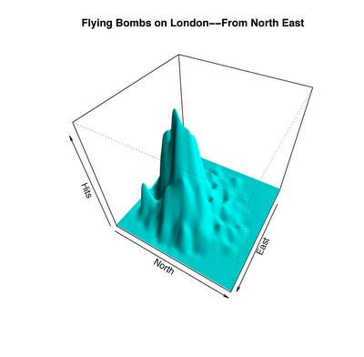
This is far from a uniform distribution, but is this evidence of accurate targeting? At the moment, you can guess how to answer this question. In a report titled “Applying the Poisson Distribution,” a British statistician named after RD Clark wrote:

During the aerial bombardment on London, it was believed that the target points of bombs, as a rule, form clusters. Therefore, it was decided to apply a statistical test to find out whether this statement is correct.

Clark took an area of ​​12 km x 12 km, which was heavily bombarded, and divided it with a grid. As a result, he got 576 squares, each 25 urban blocks. Then he calculated the number of squares with 0 bombs dropped, with the 1st bomb dropped, with 2, and so on.

A total of 537 bombs fell on these 576 squares. This is about one bomb per square average. He substituted these numbers into the Poisson formula to find out how many clusters are expected to get at random. Here is the corresponding table from his article:


Compare the two columns, and you can see how incredibly accurate prediction corresponds to reality. There are 7 squares that were hit by 4 bombs each - this is what you would expect due to chance. In most of London, the bombs did not please. They collapsed at random, in a destructive city game of Russian roulette.

Poisson distribution has the habit of sneaking up in all sorts of places, in some cases insignificantly, and in others changing your life. The number of mutations in the DNA and the age of your cells; the number of cars in front of you at the traffic lights, or patients waiting in line in front of you in the emergency room; the number of typos in each of my blog posts; the number of patients with leukemia in a given city; the number of births and deaths, marriages and divorces, or suicides and murders in a given year; number of fleas on your dog.

These Victorian scholars have taught us that from worldly moments to questions of life and death, chance plays a stronger role in our life than we are willing to admit. Unfortunately, this fact does not give consolation when the cards in the waterfall of life are distributed not in our favor.

“So much life, it seems to me, is determined by sheer chance.” - Sidney Poitier