Constructing fractal shapes in Matlab
“Iteration from person. Recursion from God. ”L. Peter Deutsch
Many of us have heard about fractals, I think that many even have a fairly clear idea of these amazing mathematical objects and their close relationship with physical natural structures. However, in this article I would like to touch on the research and philosophical aspects of this issue. By itself, the ability to generate complex patterns on the complex plane with the help of simple mathematical expressions is very tempting, in fact, it prompted writing an article. By writing a couple of lines of code, we can fall to the very bottom of the bit grid of our PC, studying scalable fractal patterns.
In one of the programs of the BBC cycle (The Secret Life of Chaos) an interesting idea was positioned, it was certainly not positioned by the authors of this video, but by Alan Turing and the father of chaos theory Edward Lorenz. As it turned out, complex systems, with a large number of links and elements (even monotonous) have a threshold of predictability. What does it mean? The combination of the simplest structures with deterministic logic can yield very, very complex behavior at the output. Almost so it turns out in our case: taking the simple recurrence relation Z [i + 1] = Z [i] ^ (n) + C, i = 1, 2, ... inf where C is a complex number, Z [0] = 0 , we will see that some sums will be finite, and some will run off to infinity (depending on the chosen C). Below is the code, it will be clearer. Of great interest is the behavior of points on the boundary of divergence. They form complex, sometimes self-repeating patterns that can change with increasing degree of scaling, generating an endless dynamic pattern. Sometimes it is interesting to watch these drawings, by changing the degree of a polynomial, or by putting new functions in a recursive formula, you can get very interesting pictures.
Let's start by writing the script fractal.m: Let's set the size of the image to be 500x500 pixels, the area [-2, 1] will be interesting for us; on the real axis and [-1.5, 1.5]; along the imaginary axis, in it we will observe a fractal. If the sum of the series goes beyond the boundaries of this square, then we consider that the series diverges.
')
Next, we draw a fractal using the draw_fractal function, we will look at it later. It takes the bounding box and the size of the image at the entrance. This function returns the recalculated pixel sizes in the enlarged area i.e. pb_re pb_im is the mathematical size of a pixel along the imaginary and real axis. Next, we select the area to be approximated via getrect , current_point , the left upper point of the zoom rectangle, we get the width and height of the bounding rectangle specified by the mouse. bound_re and bound_im new boundaries of the area under consideration (similar to the initial). Then everything repeats.
The draw_fractal.m function calculates what mathematical size pixel_bounds_re and pixel_bounds_im pixel corresponds to, then we go over the image matrix and consider the mathematical set of points lying in the center of our pixel boxes, for each point using the [color] = is_a_m_point (current_point) function, we calculate the running away whether it is infinite or not.
And the faster the point will run away to infinity, the brighter it will be, it can be seen from the function is_a_m_point.m. It accepts our constant C from the recursive formula Z [i + 1] = Z [i] ^ (n) + C , the problem the function is to return the color color - the faster the row diverges the brighter the color, if the point runs out of the boundaries [-2 1] (real axis) [-1.5 1.5] (imaginary axis), then we believe that the row diverges . We believe that Z [0] = 0, and in the series we add 50 numbers (as a rule, this is enough to understand whether the series will diverge or not).
That's all. Having written a couple of scripts you can relax and try to explore what happened as a result. Since the poor set of Mondelbrot already where it is not even glowing, we will try to investigate something more interesting, for example, the function z = z ^ (2) / (1 + z + z ^ (4)) + constant;
This dependence generates the following figure on the complex plane:

The left central part of this picture is interesting because by bringing it closer we will fall into an endless renewing pattern of self-similar figures. A beautiful allegory to the fact that the variety can be generated by a group of finite primitives.
Using the presented Matlabov scripts, it is easy to get and the dynamics of changes in fractal patterns on the plane, for example, changing the degree of the polynomial n in the recursive formula Z [i] = Z [i-1] ^ (n) + C, n = 1, 2 ... 200, you can get the following
http://video.yandex.ru/users/alexhoppus/view/2/
In this article I tried to present the simplest version of the implementation of scripts in the Matlab environment, creating fractal patterns of arbitrary recursive dependence with the possibility of scaling. It is easy to see that each dependence creates in its own way a unique world on a complex plane, with its own “laws of pattern formation”, with its own symmetry. From all this you can make a lot of intuitive reasoning, some of which I have already cited in the text of the article. In the cycle of his lectures, Franklin Merrell-Wolf (Mathematics, philosophy of yoga) raises the question of the duality of human thinking and the human desire to fragment the reality, and also raises the question "Is it true that the world consists of something?". So is he, or is there just one recursive formula at the head of everything, which gives rise to an immense variety of reality?
Introduction
Many of us have heard about fractals, I think that many even have a fairly clear idea of these amazing mathematical objects and their close relationship with physical natural structures. However, in this article I would like to touch on the research and philosophical aspects of this issue. By itself, the ability to generate complex patterns on the complex plane with the help of simple mathematical expressions is very tempting, in fact, it prompted writing an article. By writing a couple of lines of code, we can fall to the very bottom of the bit grid of our PC, studying scalable fractal patterns.
About fractals
In one of the programs of the BBC cycle (The Secret Life of Chaos) an interesting idea was positioned, it was certainly not positioned by the authors of this video, but by Alan Turing and the father of chaos theory Edward Lorenz. As it turned out, complex systems, with a large number of links and elements (even monotonous) have a threshold of predictability. What does it mean? The combination of the simplest structures with deterministic logic can yield very, very complex behavior at the output. Almost so it turns out in our case: taking the simple recurrence relation Z [i + 1] = Z [i] ^ (n) + C, i = 1, 2, ... inf where C is a complex number, Z [0] = 0 , we will see that some sums will be finite, and some will run off to infinity (depending on the chosen C). Below is the code, it will be clearer. Of great interest is the behavior of points on the boundary of divergence. They form complex, sometimes self-repeating patterns that can change with increasing degree of scaling, generating an endless dynamic pattern. Sometimes it is interesting to watch these drawings, by changing the degree of a polynomial, or by putting new functions in a recursive formula, you can get very interesting pictures.
Code writing
Let's start by writing the script fractal.m: Let's set the size of the image to be 500x500 pixels, the area [-2, 1] will be interesting for us; on the real axis and [-1.5, 1.5]; along the imaginary axis, in it we will observe a fractal. If the sum of the series goes beyond the boundaries of this square, then we consider that the series diverges.
image_size = 500; bound_re = [-2, 1]; bound_im = [-1.5, 1.5]; ')
Next, we draw a fractal using the draw_fractal function, we will look at it later. It takes the bounding box and the size of the image at the entrance. This function returns the recalculated pixel sizes in the enlarged area i.e. pb_re pb_im is the mathematical size of a pixel along the imaginary and real axis. Next, we select the area to be approximated via getrect , current_point , the left upper point of the zoom rectangle, we get the width and height of the bounding rectangle specified by the mouse. bound_re and bound_im new boundaries of the area under consideration (similar to the initial). Then everything repeats.
while(1) [pb_re pb_im] = draw_fractal(bound_re, bound_im, image_size); rect = getrect; current_point = complex(bound_re(1) + rect(1) * pb_re - 0.5 * pb_re , ... bound_im(1) + rect(2) * pb_im - 0.5 * pb_im); current_width = rect(3) * pb_re; current_height = rect(4) * pb_im; bound_re = [real(current_point), real(current_point) + current_width]; bound_im = [imag(current_point), imag(current_point) + current_height]; end The draw_fractal.m function calculates what mathematical size pixel_bounds_re and pixel_bounds_im pixel corresponds to, then we go over the image matrix and consider the mathematical set of points lying in the center of our pixel boxes, for each point using the [color] = is_a_m_point (current_point) function, we calculate the running away whether it is infinite or not.
function [pixel_bounds_re, pixel_bounds_im]=draw_fractal( bound_re, bound_im, image_size) pixel_bounds_re = (bound_re(2) - bound_re(1) ) / image_size; pixel_bounds_im = (bound_im(2) - bound_im(1) ) / image_size; frac = zeros([image_size, image_size]); parfor re = 1 : image_size for im = 1 : image_size current_point = complex(bound_re(1) + re * pixel_bounds_re - 0.5 * pixel_bounds_re , bound_im(1) + ... im * pixel_bounds_im - 0.5 * pixel_bounds_im); [color] = is_a_m_point(current_point); frac(im,re) = color; end end frac = mat2gray(frac); imshow(frac); end And the faster the point will run away to infinity, the brighter it will be, it can be seen from the function is_a_m_point.m. It accepts our constant C from the recursive formula Z [i + 1] = Z [i] ^ (n) + C , the problem the function is to return the color color - the faster the row diverges the brighter the color, if the point runs out of the boundaries [-2 1] (real axis) [-1.5 1.5] (imaginary axis), then we believe that the row diverges . We believe that Z [0] = 0, and in the series we add 50 numbers (as a rule, this is enough to understand whether the series will diverge or not).
function [ color] = is_a_m_point( constant ) color = 0; z = 0; % Z[0] for i = 1 : 50 z = z^(2) / (1 + z + z^(4)) + constant; % if real(z) < -2 || real(z) > 1 || imag(z) > 1.5 || imag(z) < -1.5 color = 255 - 5.5 * (i - 1); return; end end end That's all. Having written a couple of scripts you can relax and try to explore what happened as a result. Since the poor set of Mondelbrot already where it is not even glowing, we will try to investigate something more interesting, for example, the function z = z ^ (2) / (1 + z + z ^ (4)) + constant;
Visualization
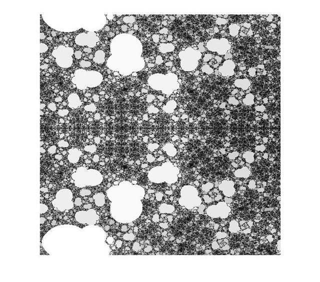
This dependence generates the following figure on the complex plane:
The left central part of this picture is interesting because by bringing it closer we will fall into an endless renewing pattern of self-similar figures. A beautiful allegory to the fact that the variety can be generated by a group of finite primitives.
Using the presented Matlabov scripts, it is easy to get and the dynamics of changes in fractal patterns on the plane, for example, changing the degree of the polynomial n in the recursive formula Z [i] = Z [i-1] ^ (n) + C, n = 1, 2 ... 200, you can get the following
http://video.yandex.ru/users/alexhoppus/view/2/
Conclusion
In this article I tried to present the simplest version of the implementation of scripts in the Matlab environment, creating fractal patterns of arbitrary recursive dependence with the possibility of scaling. It is easy to see that each dependence creates in its own way a unique world on a complex plane, with its own “laws of pattern formation”, with its own symmetry. From all this you can make a lot of intuitive reasoning, some of which I have already cited in the text of the article. In the cycle of his lectures, Franklin Merrell-Wolf (Mathematics, philosophy of yoga) raises the question of the duality of human thinking and the human desire to fragment the reality, and also raises the question "Is it true that the world consists of something?". So is he, or is there just one recursive formula at the head of everything, which gives rise to an immense variety of reality?
Source: https://habr.com/ru/post/162725/
All Articles