Multithreading and Task Analysis in Intel® VTune ™ Amplifier XE 2013

One of the methods for improving the efficiency of parallelization of algorithms of a certain class is the pipelining of execution phases, both sequential and parallel. The Intel TBB Library can help reduce the effort and time required to implement pipelined algorithms, taking care of task management and load distribution between threads in the system. However, the formulation and formation of tasks that make up the phases of an algorithm can be a non-trivial problem, depending on the complexity of the algorithm, which often happens in real-world applications. It may be even more difficult to control the execution of tasks if the algorithm itself does not contain means for control. The toolkit for analyzing computational tasks in Intel VTune Amplifier helps developers present the structure of execution in a multi-threaded environment in a convenient graphical form, increasing the efficiency of analysis and significantly reducing the time to develop applications. In this article, we will look at a simple example of a pipelined task, and step by step we will parallelize it using the TBB pipeline class, analyze it using the VTune Amplifier, and improve the performance of the implementation based on the analysis results.

Introduction

As is known, a computational task in general can be divided into subtasks (decomposition), which are performed in parallel by different computing devices. Depending on the type of task, or input data, decomposition can be applied to the data, or to the task itself. Simply put, data decomposition can be considered as separating the input dataset for processing by the same algorithm, but in different calculators. Decomposition into tasks is, on the contrary, several different algorithms executed by different devices, either on the same data or on different parts of them. The main purpose of decomposition for computing devices is to ensure that all available devices are as busy as possible all the time while the task is being calculated. This achieves maximum performance for the existing set of devices when performing this task, which means reducing the time to complete it. In this regard, the ability to analyze the implementation of both each part of the task and the task as a whole in the computing system is of great importance for the optimization of the algorithm. In this article, we consider the analysis of computational tasks parallelized using the Intel TBB library using the new version of the VTune Amplifier XE 2013 profiler.

Immediately I will ask to excuse me for the abundance of English terms without translation. This was done intentionally, because using the tools you still have to use them, and attempts to translate them into Russian will only confuse the reader. (UPD: I was told that the untranslated text in the pictures hurts my eyes - I work on the translation and will update the pictures soon)

The introduction does not accidentally contain an abundance of generalizing expressions, such as a computer system, a data set, etc., because we start with a generalized example that has little to do with real-world tasks, and then gradually move on to a living example, which we analyze . Let's consider a spherical algorithm that runs in a vacuum, but it strongly resembles the real task of obtaining data from any source, performing some sorting procedures on this data, and writing the processed data to the receiver (Fig. 1). This structure is quite typical for many applications, among which, codecs, filters, or communication protocols most quickly come to mind.
')

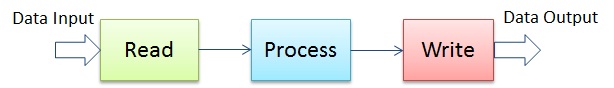
Pic1

To maintain the depth of the vacuum and simplify the example, we will not take into account the possible relationship between the parts of the data coming from the source. Although this is not correct, as, for example, when processing video frames in a codec, the dependence of neighboring pixels is taken into account by the algorithm. However, in the general case, one can always isolate a sufficiently large data array, which can be considered independent of other arrays. At the same time, it is quite safe to apply decomposition to execute a computational algorithm in parallel over different parts of the data, thereby distorting the sphericity of the algorithm and making something similar to the scheme shown in Fig. 2: the data are sequentially read from the source, processed in parallel blocks (P) , and then again sequentially recorded (W) at the receiver.


Pic2

If the data source is a serial device, such as a disk, or a network interface, then the process of reading and writing will also be sequential. And even if you have free computing threads in the system, the only stage of execution that can be parallelized is the execution phase of the algorithm. According to Amdal's law , the increase in the performance of the entire task due to parallelization will be limited to these successive phases.

Trying to overcome this limitation, we can redistribute parts of the task in such a way as to ensure that all executive threads are constantly busy with its execution. This is possible if parts of the data are independent and their processing order is not important, or can be restored at the output. To do this, we build a simple pipeline that consists of the same Read / Process / Write stages performed by each thread (Figure 3). The Read and Write stages are still consistent, but they are distributed between the threads. It should be borne in mind that no thread can begin the stage of reading or writing, while any other thread performs the same stage. However, two different threads can quite simultaneously perform both reading and writing different data.


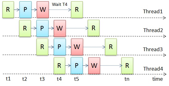
Pic.3

Having restructured the algorithm in such a way, formally we used decomposition by tasks, that is, different phases of the task were performed by different threads simultaneously. At the same time, dividing data into parts, and performing the same operations on them in different streams, we use data decomposition. Such a combined approach allows us to ensure that the threads are constantly busy working, thereby maximizing the efficiency of the execution of the entire task. However, the sphericity of the algorithm still remains the same, since we do not take into account possible delays in the read / write devices, and also assume that there is a lot of work for computational flows to smooth out irregularities in the data input, and computing devices are always available for execution algorithm.

In real life, things can be more complicated. For example, no one guarantees a stable value of the time spent by input / output devices for data transfer, or that the processors are free at the moment, or that the data is homogeneous and require the same time to be processed by the same algorithm. Most often, the input data may arrive with a delay, due to the peculiarities of the source. The processor may be busy with other tasks with a higher priority. Some data may require more processing time, for example, frames with fine details are processed much longer by a compression algorithm than frames with a uniform background. Recording operations are usually not a problem, since in most systems they are buffered and physically recording data to the receiver can be delayed until later. Although this only works if the output is not used again at the input. In general, moving from a spherical-vacuum model to real implementations of the problem in the existing system, all conceived efficiency of the conveyor may come to naught, and our complex scheme will remain as ineffective as was the original and simple (Figure 4).


Pic.4

To eliminate the inefficiencies that have arisen due to load imbalances, we can try to dynamically distribute the work performed by each thread. This will require monitoring the employment status of the streams, managing the size of the data processed by the algorithm, and distributing the subtasks among the free streams. The implementation of such an infrastructure is possible with small efforts, but only for simple cases. In general, such an infrastructure can be quite complex to develop from scratch. And then it's time to advertise the capabilities of the Intel TBB library, which already contains a mechanism for dynamic load balancing between threads. And for our example, TBB contains a built-in pipeline algorithm called the pipeline class , suitable for use in our task.

Example

We will not go into much detail about the implementation of the pipeline algorithm in TBB, since all the information, including open source, can be found at threadingbuildingblocks.org . Below, we will simply take an example of our task, how to create a pipeline using TBB. A sample of the code is in the library directory or on the website.

In a nutshell, a pipeline is the application of a sequence of execution units to a stream of objects. Executive units can implement stages of the task that perform certain actions on the data stream. In the TBB library, these stages can be defined as instances of the filter class. Thus, the pipeline is built as a sequence of filters. Some stages (such as Processing) can work in parallel in several streams with different data, so they must be defined as parallel filter Class. The remaining stages, such as Read and Write, must be performed sequentially and in a specific order (if the order change is not provided), and we define them as the serial_in_order filter Class. The library contains abstract classes for these types, and we need to inherit our classes from them. Below is an example that, with certain simplifications, shows how to do this.

class MyReadFilter: public tbb::filter { FILE* input_file; DataItem* next_item; /*override*/ void* operator()(void*); public: MyReadFilter( FILE* in ); };	MyReadFilter:: MyReadFilter( FILE* in ) : filter(serial_in_order), input_file(in), next_item(DataItem*) { }
class MyWriteFilter: public tbb::filter { FILE* output_file; /*override*/ void* operator()(void*); public: MyWriteFilter( FILE* out ); };	MyWriteFilter:: MyWriteFilter( FILE* out ) : filter(serial_in_order), output_file(out), { }

In our example, the data is contained in a file, so you need to define a private member of the class for the file pointer. Similarly, we define the MyWriteFilter class for the write stage, and store the pointer to the output file. These classes will be responsible for allocating memory for the data and passing objects along the pipeline. The main work is performed in the operator () method defined in the base class. We only need to override these methods by implementing accordingly reading data from the input file to the container and writing data from the container to the output file.

void* MyReadFilter::operator()(void*) { // ALLOCATEMEMORY // READ A DATA ITEM FROM FILE // PUT DATA ITEM TO CONTAINER }

void* MyWriteFilter::operator()(void*) { // GET DATA ITEM FROM CONTAINER // WRITE THE DATA ITEM TO FILE // DEALLOCATE MEMORY }

Our Process stage can run in parallel in streams, therefore we define it as a parallel filter class, and the operator () method should contain the “meat” of the data stream processing algorithm.

class MyProcessFilter: public tbb::filter { public: MyProcessFilter(); /*override*/void* operator()( void* item ); }; MyProcessFilter:: MyProcessFilter() : tbb::filter(parallel) {}

void* MyProcessFilter::operator()( void* item ) { // FIND A CURRENT DATA ITEM IN CONTAINER // PROCESS THE ITEM }

It remains for us only to finally assemble the pipeline: create objects of the class filter , an object of the class pipeline , and connect all the stages. After building the pipeline, you must call the run () method of the class class pipeline , specifying the number of tokens (sorry for such a transfer). In this case, the number of tokens means the number of data objects that can be executed in the pipeline simultaneously. Choosing the right amount can be a separate topic for discussion, we simply follow the recommendations in the documents for TBB and choose a number equal to twice the number of streams available in the system. This will give us the opportunity to have enough data objects to keep the pipeline busy and, at the same time, ensures that the queue of data objects does not grow if the first stage processes them much faster than subsequent ones.

  tbb::pipeline pipeline; MyReadFilter r_filter( input_file ); pipeline.add_filter( r_filter ); MyProcessFilter p_filter; pipeline.add_filter(p_filter ); MyWriteFilter w_filter( output_file ); pipeline.add_filter( w_filter ); pipeline.run(2*nthreads) 

Thus, we created three subtasks in the pipeline that will be controlled by the TBB library to maximize the use of processors available in the system - the Process subtask will be parallelized, and the remaining subtasks will be dynamically distributed between threads depending on their availability. We only needed to correctly connect these stages. As you can see, in the example there is no flow control code — all of this is hidden in the library's task scheduler.

And as is often the case, somewhere in the next-to-last series (or, vice versa, from the first), a hand rises, and a very meticulous listener asks a very good question: How can we be sure that the constructed conveyor is efficient? And if you dig deeper, how do you know how exactly the subtasks are performed in the pipeline, and what are the overhead costs of managing subtasks, and are there any gaps in their execution?

It is meaningless to suggest comparing its implementation with the original, inefficient implementation of the algorithm. First, so we will not understand anything, except that it will work faster. And secondly, it is possible that it will work faster and will not.

That is, there are no simple answers to the questions posed. Need to measure and analyze. Profiling with VTune Amplifier XE will make this process easier, more visual, and most importantly, fast. VTune Amplifier will help us determine the efficiency of loading processors in the system, visually show the TBB task management scheme, and detect possible errors that we made in the process of constructing the pipeline that affect the performance of the algorithm implementation.

Let's start with Hotspot analysis for educational purposes. We will analyze an example of code that reads integer values ​​from a file in text format [Read stage], squares them in [Process] and writes numbers in text format to the [Write] output file. We will assume that the reader is familiar with the basics of working with the VTune profiler, and will not go into details, which button to press to start the profiling.


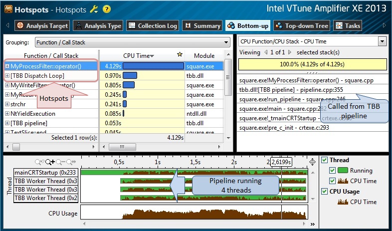
Fig.5.

The results of the Hotspot analysis (Fig. 5) are quite expected - the test program was executed in 4 threads on a 4-core processor; The MyProcessClass :: operator () method, called from the TBB pipeline, is the hottest function, since it converts from a text to an integer value, calculates the square of the value, and performs the inverse conversion to text. Interestingly, some function [TBB Dispatch Loop] (not really a function, but a conventional name that hides the “insides” of the TBB scheduler) is also on the hot list, which can tell us about the possible presence of planning overheads. Let's continue with the Concurrency analysis so far, and determine the efficiency of the algorithm parallelization.


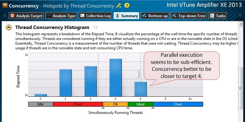
Fig.6.

From the resulting histogram of parallelism of the program, we see that we are far from maximum efficiency: in general, the application was executed in less than 4 streams. (The blue bars in the histogram show on the Y axis how long the application worked in X threads. Ideally, we would like to see a single bar with a parallelism level of 4 [concurrency level4], which would mean that our application was working in 4 threads all the time) .
Even a quick glance at the results in the Bottom-Up View is enough to see the redundant synchronization that occurred between the threads (Fig. 7). You can hover the mouse on the yellow lines of the transition control (transitions) and see in the pop-up window a link to the source of this synchronization.


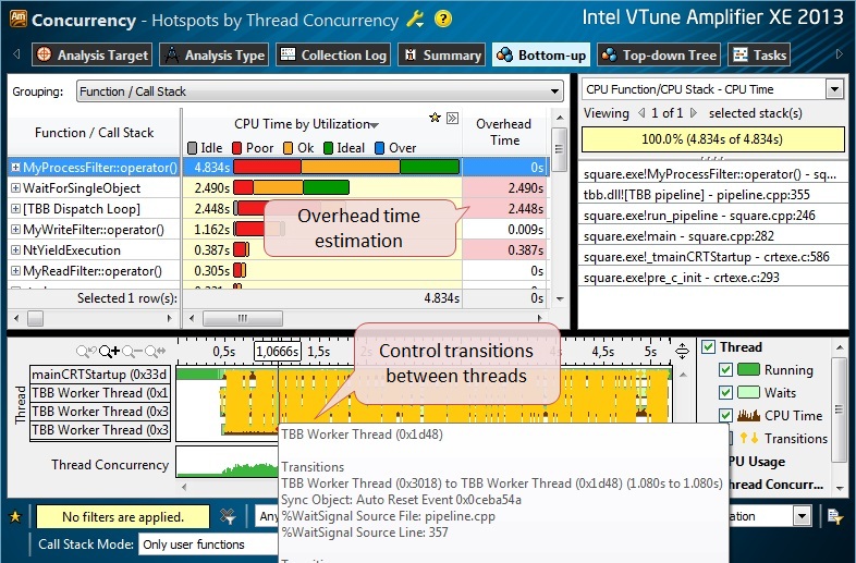
Fig.7.

At this point, even the most patient user would have thrown further research, incidentally accusing the developers of TBB in an inefficient implementation of the library. I would have done the same thing if I didn’t have a tool at hand to analyze the work of the scheduler. Theoretically, one can imagine the independent tracing of tasks using source code instrumentation, and parsing the trace “manually” or using some script to identify the time relationships of the tasks. However, this path does not look attractive because of the laboriousness of processing the collected trasses. Therefore, I advise you to use a toolkit that already exists in VTune Amplifier and which can be used to quickly restore the structure of user tasks in a convenient graphical form.

To enable the task analyzer, we need to instrument the source code using special functions from the Task API, which is available in VTune Amplifier. Listed below are the steps you need to do to do this:

1. Include the header file from the User API in your source
   

    #include "ittnotify.h" 

2. Determine the domain of the task. It is often very convenient to separate tasks performed in different domains, for example, threads in different parallel infrastructures (TBB, OpenMP, etc.)
   

    __itt_domain* domain = __itt_domain_create("PipelineTaskDomain"); 

3. Identify the task descriptor that describes the stage.
   

    __itt_string_handle* hFileReadSubtask = __itt_string_handle_create("Read"); __itt_string_handle* hFileWriteSubtask = __itt_string_handle_create("Write"); __itt_string_handle* hDoSquareSubtask = __itt_string_handle_create("Do Square"); 

4. Now wrap the source code, executed in the task stages, with calls to the instrumental API functions: __itt_task_begin and __itt_task_end . For example, the read and write stages can be interpreted as follows:
   

    void* MyReadFilter::operator()(void*) { __itt_task_begin(domain, __itt_null, __itt_null, hFileReadSubtask); // ALLOCATE MEMORY // READ A DATA ITEM FROM FILE // PUT DATA ITEM TO CONTAINER __itt_task_end(domain); } 

   
   

    void* MyWriteFilter::operator()(void*) { __itt_task_begin(domain, __itt_null, __itt_null, hFileWriteSubtask); // GET DATA ITEM FROM CONTAINER // WRITE THE DATA ITEM TO FILE // DEALLOCATE MEMORY __itt_task_end(domain); } 

   
   Likewise, you can wrap and the stage of processing numbers (Process stage). (Further information on User API functions can be found in the product documentation).
   

    void* MyProcessFilter::operator()( void* item ) { __itt_task_begin(domain, __itt_null, __itt_null, hDoSquareSubtask); // FIND A CURRENT DATA ITEM IN CONTAINER // PROCESS THE ITEM __itt_task_end(domain); } 

   
   
5. Do not forget to add the path to the VTune Amplifier header files to your project:
   $ (VTUNE_AMPLIFIER_XE_2013_DIR) include
6. Statically link your executable with the library libittnotify.lib , the path to which is located
   $ (VTUNE_AMPLIFIER_XE_2013_DIR) lib [32 | 64] depending on the “bitness” of your system.

Finally, it remains for us to enable the analysis of user tasks in the analysis configuration window (Fig. 8) and run any type of profiling that we need.


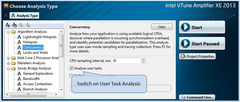
Fig.8.

After the Concurrency profiling is finished, we switch to the Tasks View tab (Fig.9). Here, we are somewhat hampered by the yellow lines of flow control transitions - they can be turned off in the panel to the right, as are the CPU Time graphics, which may close the necessary information. However, even with this, tasks are poorly distinguishable on a timeline; color bars representing a graphic representation of tasks are too thin to distinguish them. In this case, select the smaller time interval and zoom in (Zoom-In) from the context menu by right-clicking the mouse, or using the toolbar.


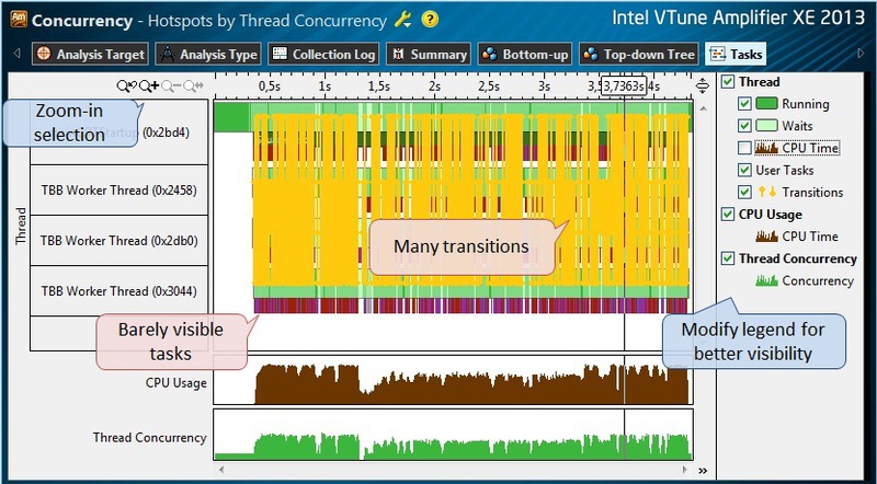
Fig.9.

In the enlarged image of the tasks we can notice a couple of problems (Fig. 10). The first is the huge (compared to the duration of the tasks themselves) intervals between tasks, during which the threads are in an inactive state, that is, the processors are idle waiting for synchronization events. The second problem is the duration of the task phases. For example, the “Do Squire” subtask is only about 0.1 milliseconds. This is a critically small execution interval, given that the tasks are managed by the TBB scheduler, and it takes some time to plan and assign them to workflows (TBB Worker Thread). That is, it turns out that the overhead of managing subtasks is commensurate with the execution time of the task itself. This should not be allowed, so it is necessary to increase the time spent on work in the subtask, that is, in other words, give it more work.


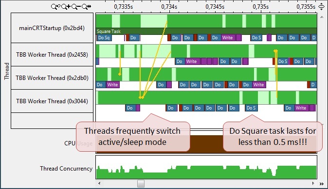
Fig. ten.

In our example, it is already clear what functions in the code perform what tasks, but this was done intentionally to simplify the presentation in the article. In a real-world application in the execution of tasks dozens of functions can be involved. To find all the functions that influenced the execution of tasks, and increase their workload, we can switch to the Bottom-Up view results for Concurrency, or the Hotspot profiling. Now we simply change the grouping of functions by task type (TaskType / Function) and get in the table a list of subtasks that we created by instrumenting the application. Opening the task, clicking on the “+” icon, we get a list and a tree of function calls that participated in the execution of this subtask, occupying a statistically significant processor time (Fig. 11).


Fig.11.

Next, by double-clicking, we go to the source code of the hot function MyProcessFilter :: operator () and find that it works with a text segment transmitted to it (text slice) (Fig. 12). Inside this function, it iterates over characters in the text, converts to an integer type, multiplies the value by itself, and converts it back to a text character. The most obvious way to increase the load for this subtask would be to increase the size of a piece of text — this will linearly increase the number of operations performed in this subtask. We simply choose the new size of the maximum number of characters in the MAX_CHAR_PER_INPUT_SLICE segment, which will be, say, 100 times greater than the original (based on the time indicators we received during the profiling). We also assume that the efficiency of read and write operations will also increase with increasing data size for a single object.


Fig.12.

We recompile the application and profile it again using task analysis (Figure 13). The Do Square subtask is now executed in about 10 milliseconds (hover the mouse over the task image to get numerical characteristics). There are also practically no “gaps” between the subtasks, which makes the threads occupied more time. You can also notice how the TBB scheduler builds up the same, but shorter subtasks, such as the Write phase, connecting them into a longer queue, and assigning them to execute in one thread, thereby reducing the cost of additional synchronization.


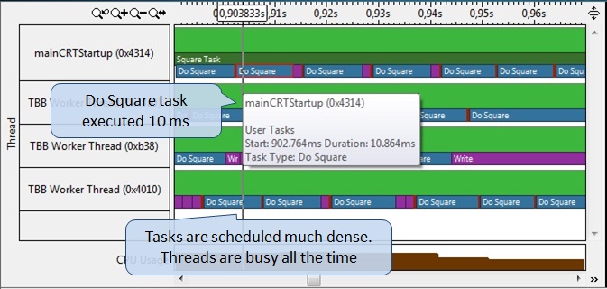
Fig.13.

It will also be interesting for us to check the total parallelism throughout the program. As can be seen in Figure 14, the application was performed mainly by 3 or 4 threads, which is a significant achievement compared to the initial results. You can also compare the average value of the Concurrency Level, but you need to remember that it affects the sequential part of the application, including the one that we did not parallelize.

Yes, the serial part of the program remains, but it has decreased by a third. It can also be seen in the results in TimeLine View. If we select this sequential part and filter the rest of the time, then we can see that it corresponds to the initialization phase of the entire application in the main thread. If we want to determine exactly what part corresponded to the work of the pipeline and does not relate to initialization, then we can use the User API functions that control the profiling — starting the collection immediately before creating the conveyor, and ending the collection after doing the work.


Fig.14.

In addition to graphs that give an estimate of the improvement in the efficiency of implementation, we can see and compare the numerical indicators of application performance. All results in VTune Amplifier can be compared using the corresponding comparison functionality. I will simply bring two pictures side by side, for a better perception of the compliance of the results of the initial Hotspots analysis, and obtained after changing the code (Figure 15). What is interesting, although the program execution time (Elapsed Time) has decreased, the time spent in the MyProcessFilter :: operator () function has not changed, since we have not changed the total amount of work, but it has simply been redistributed. At the same time, the cost of scheduling TBB tasks was significantly reduced. In addition, the total time of reading and writing data also decreased, obviously, due to more efficient work with large segments of text.


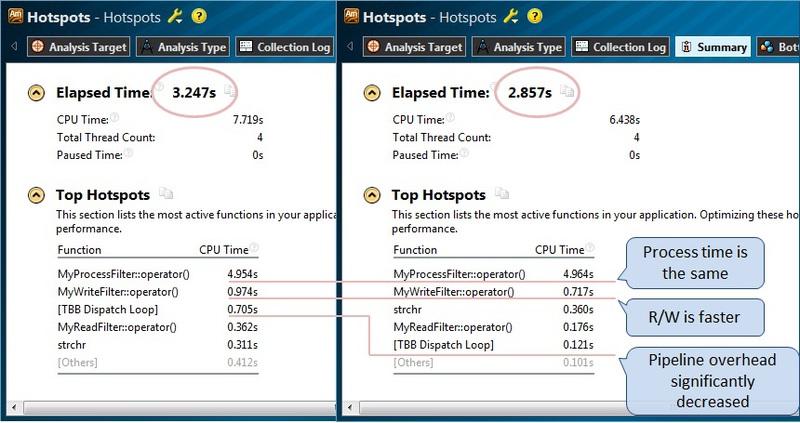
Fig.15.

Conclusion

Data and task decomposition is effectively used for parallelization of algorithms. Some classes of algorithms can be improved by using the method of pipelining sequential and parallel phases of execution. The Intel TBB library can help significantly reduce the time required to implement pipelining algorithms, while taking on the task of scheduling tasks and balancing their execution in the streams available in the system. Formation of tasks based on the phases of the algorithm can be a non-trivial task, depending on the complexity of the implemented algorithm, and managing the execution of tasks can be even more difficult. VTune Amplifier’s Task Analysis toolkit helps developers present the structure of task execution in a multi-threaded environment in a convenient graphical form, increasing analysis efficiency and significantly reducing application development time.