Speech Preprocessing with Matlab
The result of pre-processing of speech signals is to obtain a set of spectral vectors characterizing this signal and are used for further recognition.
The fundamental assumption that is made in modern discriminators is that the speech signal is regarded as stationary (that is, its spectral characteristics are relatively constant) over an interval of several tens of milliseconds. Therefore, the main function of preprocessing is to divide the input speech signal into intervals and to obtain smoothed spectral estimates for each interval.
The typical value of a single interval is 25.6 ms. Neighboring intervals are taken with an offset from the previous interval. The applied overlap interval is 10 ms. As a result of preliminary study of each of these intervals, we obtain a vector of several tens of spectral values.
')
The block diagram of the speech pre-processing algorithm is shown in Fig.1.
As an example, we consider speech samples sampled at a frequency of 16 KHz and with a bit width of 16 bits. The discretized speech signal is divided into intervals of 25.6 ms duration, that is, 409 samples. Intervals overlap with a shift of 10 ms (160 samples).
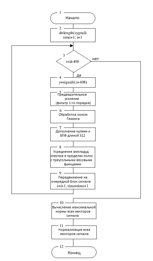
Fig.1. The block diagram of the algorithm pre-processing of the speech signal
Mel-scale is introduced to approximate the frequency separation of the human ear, which is linear up to 1000 Hz and logarithmic over 1000 Hz.
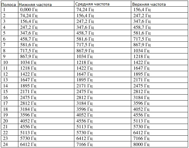
The first amplitude coefficient — the constant component of the spectrum — is ignored, and the amplitudes of the remaining 255 spectral values are averaged. Averaging is implemented as 24 triangular band-pass filters. The lower, middle and upper frequencies of such bands are presented in Table 1.
Each triangular filter finds a weighted average of those amplitude spectral values corresponding to frequencies between the lower and upper frequency for a given filter. If the amplitude corresponds exactly to the center frequency of the band, then it is multiplied by a factor of one. When moving the corresponding amplitude value of the frequency from the middle to the lower or upper limit, the coefficient decreases from one to zero.
The resulting amplitude products by coefficients are added and divided by the number of amplitude values. As a result, we find the weighted average for this frequency band.
256 amplitudes correspond to frequencies from 0 Hz to 8000 Hz, i.e. the step of movement is equal 8000/256 = 31,25 Hz. This means that the first amplitude corresponds to the frequency of 0 Hz, the second to 31.25 Hz, the third to 62.5 Hz, etc.
For example, for the first Mel-scale frequency band: the lower frequency is 0 Hz, the average frequency is 74.24 Hz, the upper frequency is 156.4 Hz.
So, the first (0 Hz), the second (31.25 Hz), the third (62.5 Hz), the fourth (93.75 Hz), the fifth (125 Hz) and the sixth (156.25 Hz) fall into the first frequency band amplitudes.
According to Fig.2. the third amplitude corresponds to a coefficient equal to 62.5 / 74.24 ≈ 0.84; and the fifth amplitude - the coefficient is (156.4-125) / (156.4-74.24) ≈ 0.38.
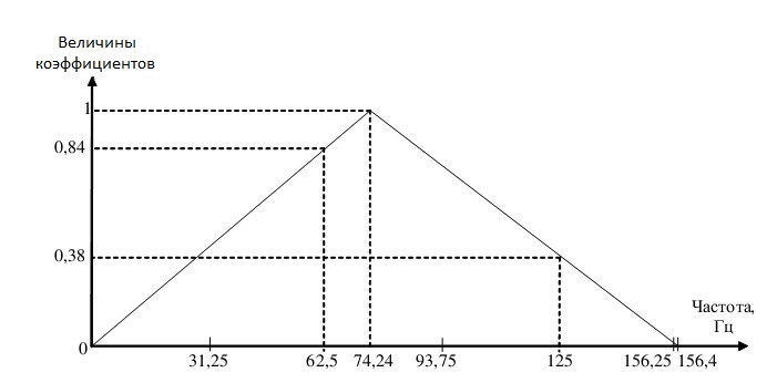
Fig.2.
Table 1 Mel-frequency scale
As a result of the described actions, we obtain a 24-element spectral (acoustic) vector.
In conclusion, we perform the normalization of acoustic vectors within a single language sample. To do this, we find the greatest length of the vector and the values of all vectors are multiplied by the reciprocal of this length.
For the simulation of the speech pre-processing algorithm, the MATLAB environment was chosen.
An illustration of stages 1-5 of pre-processing a speech signal is shown in Fig.3.
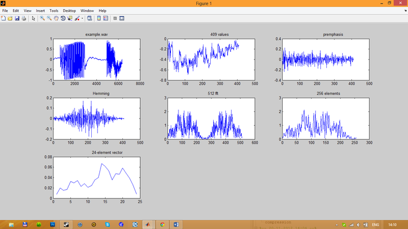
Fig.3. Speech pre-processing steps
The first illustration shows the language signal of example.wav, Discretized at 16 KHz and 16 bits.
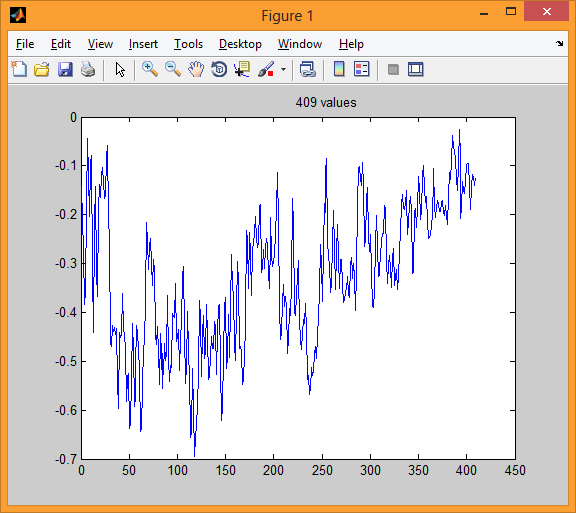
In the second illustration, we have one block (interval) of the specified speech signal with a duration of 25.6 ms. This block corresponds to 409 samples.
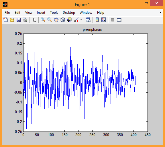
In the third illustration we see one speech signal block after processing it with a first-order filter.
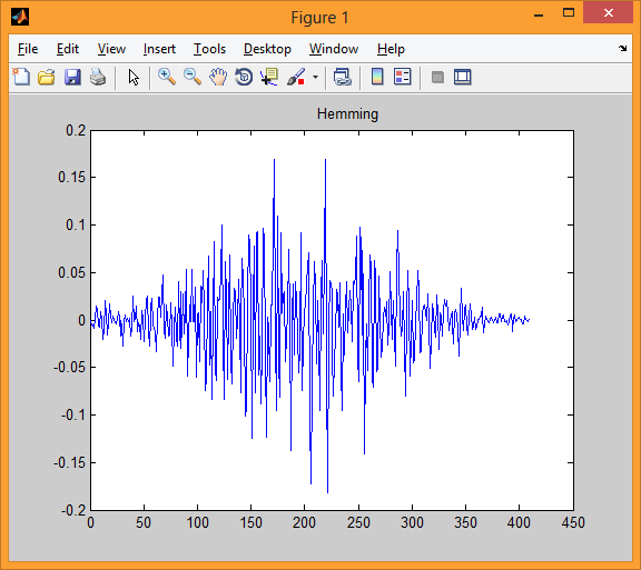
The fourth model shows us one block after applying the Hamming window.
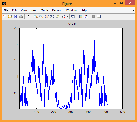
The fifth illustration gives us 512 amplitude values of the fast Fourier transform of this single block.
Since these amplitude values of the fast Fourier transform coincide in pairs (for the corresponding complex values of the fast Fourier transform are pairwise complex conjugate), it is possible to take only 256 first amplitude values. These 256 amplitude values are reflected in the sixth illustration.
The seventh illustration gives the value of a 24-element vector, the components of which are obtained after averaging 256 amplitude values within 24 “triangular” frequency bands.
The fundamental assumption that is made in modern discriminators is that the speech signal is regarded as stationary (that is, its spectral characteristics are relatively constant) over an interval of several tens of milliseconds. Therefore, the main function of preprocessing is to divide the input speech signal into intervals and to obtain smoothed spectral estimates for each interval.
The typical value of a single interval is 25.6 ms. Neighboring intervals are taken with an offset from the previous interval. The applied overlap interval is 10 ms. As a result of preliminary study of each of these intervals, we obtain a vector of several tens of spectral values.
')
The block diagram of the speech pre-processing algorithm is shown in Fig.1.
The steps that are necessary to perform for the preliminary study of each interval of the speech signal are described in detail below.
As an example, we consider speech samples sampled at a frequency of 16 KHz and with a bit width of 16 bits. The discretized speech signal is divided into intervals of 25.6 ms duration, that is, 409 samples. Intervals overlap with a shift of 10 ms (160 samples).
Fig.1. The block diagram of the algorithm pre-processing of the speech signal
Further stages of pre-processing of speech signals.
- Digitized (sampled in time and quantized by level) speech signal is divided into blocks of 25.6 ms with an offset every 10 ms, that is, blocks of 409 samples of each block, with an offset of 160 samples.
- As a rule, high-frequency amplification is used to compensate for the attenuation caused by scattering from the lips. For this, the signal blocks are passed through a first order filter.
S (1) = 0; S (n) = y (n) -y (n-1), n = 2 ... 409,
where y n is the n-th countdown in the block. - For treatments of this type, a window function is applied to each block.
In this case, the Hamming window is taken according to the expression
D (n) = (0.54-0.46 • cos (2π • (n-1) / 408)) • S (n) for n = 1, ..., 409. - To obtain spectral estimates using the discrete Fourier transform . In this case, we increase the block length to 512 elements by adding to the right with the necessary number of zeros. After that, we apply the fast Fourier transform with a length of 512 points and we obtain 512 spectral complex values. Since the 512 values to which we apply the Fourier transform are real, the resulting spectral complex values are pairwise conjugate: the second value with 512 m, the third with
511th, etc. Therefore, the last 256 complex values of the transformation are ignored, because they are complexly linked with the previous ones and do not carry new information. - For the first 256 complex spectral values, we find their amplitudes. The Fourier amplitude spectrum is smoothed (averaged) by adding the amplitudes of the spectral coefficients within the “triangular” frequency bands located on a nonlinear (logarithmic-like) Mel scale . For the limiting frequency of a language equal to 16 KHz, 24 such frequency bands are taken.
Mel-scale is introduced to approximate the frequency separation of the human ear, which is linear up to 1000 Hz and logarithmic over 1000 Hz.
The first amplitude coefficient — the constant component of the spectrum — is ignored, and the amplitudes of the remaining 255 spectral values are averaged. Averaging is implemented as 24 triangular band-pass filters. The lower, middle and upper frequencies of such bands are presented in Table 1.
Each triangular filter finds a weighted average of those amplitude spectral values corresponding to frequencies between the lower and upper frequency for a given filter. If the amplitude corresponds exactly to the center frequency of the band, then it is multiplied by a factor of one. When moving the corresponding amplitude value of the frequency from the middle to the lower or upper limit, the coefficient decreases from one to zero.
The resulting amplitude products by coefficients are added and divided by the number of amplitude values. As a result, we find the weighted average for this frequency band.
256 amplitudes correspond to frequencies from 0 Hz to 8000 Hz, i.e. the step of movement is equal 8000/256 = 31,25 Hz. This means that the first amplitude corresponds to the frequency of 0 Hz, the second to 31.25 Hz, the third to 62.5 Hz, etc.
For example, for the first Mel-scale frequency band: the lower frequency is 0 Hz, the average frequency is 74.24 Hz, the upper frequency is 156.4 Hz.
So, the first (0 Hz), the second (31.25 Hz), the third (62.5 Hz), the fourth (93.75 Hz), the fifth (125 Hz) and the sixth (156.25 Hz) fall into the first frequency band amplitudes.
According to Fig.2. the third amplitude corresponds to a coefficient equal to 62.5 / 74.24 ≈ 0.84; and the fifth amplitude - the coefficient is (156.4-125) / (156.4-74.24) ≈ 0.38.
Fig.2.
Table 1 Mel-frequency scale
As a result of the described actions, we obtain a 24-element spectral (acoustic) vector.
In conclusion, we perform the normalization of acoustic vectors within a single language sample. To do this, we find the greatest length of the vector and the values of all vectors are multiplied by the reciprocal of this length.
For the simulation of the speech pre-processing algorithm, the MATLAB environment was chosen.
clear all; close all; signal = wavread('example.wav') ; subplot(3,3,1); plot(signal);title('example.wav'); % signal: fdyscr=16 KHz, 16 bit % acoustic preprocessing of signal d=length(signal); tim=1; i=1; while i<d-408 y=signal(i:i+408); % block processing; result - acoustic vector x(1)=0.0; for j=2:409 x(j)=y(j)-y(j-1); end; %premphasis % pi=3.14; for j=1:409 z(j)=(0.54-0.46*cos(2*pi*(j-1)/408))*x(j); end; %Hamming window C=fft(z,512); C=abs(C); % FFT S=C(1:256); % amplitudes % binning of 255 spectral values amplitudes, j=2,3,...,256 f=[0; 74.24; 156.4; 247.2; 347.6; 458.7; 581.6; 717.5; 867.9; 1034; 1218; 1422; 1647; 1895; 2171; 2475; 2812; 3184; 3596; 4052; 4556; 5113; 5730; 6412; 7166; 8000]; krok=16000/512; % krok=31,25 a(1:26)=0; j=2; k=1; n(1:26)=0; h=krok*(j-1); while k<26 while and(f(k)<h,h<f(k+1)) alfa=(hf(k))/(f(k+1)-f(k)); % interval [f(k),f(k+1)]; a(k+1)=a(k+1)+S(j)*alfa; n(k+1)=n(k+1)+1; a(k)=a(k)+S(j)*(1-alfa); n(k)=n(k)+1; j=j+1; h=krok*(j-1); end; a(k)=a(k)/n(k); k=k+1; end; O(tim,1:24)=a(2:25); %O(tim,25)=sum(y.^2); norma(tim)=norm(O(tim,1:24)); i=i+160; tim=tim+1; % next block end; % end of block proccesing time=tim-1; normamax=max(norma(1:time)); O(1:time,1:24)= O(1:time,1:24)/normamax; % normalization % end of signal acoustic preprocessing subplot(3,3,2); plot(y);title(' 409 values '); subplot(3,3,3); plot(x);title(' premphasis '); subplot(3,3,4); plot(z);title(' Hemming'); subplot(3,3,5); plot(C);title(' 512 fft '); subplot(3,3,6); plot(S);title(' 256 elements '); subplot(3,3,7); plot(O(time,1:24));title(' 24-element vector'); An illustration of stages 1-5 of pre-processing a speech signal is shown in Fig.3.
Fig.3. Speech pre-processing steps
Illustrations of processing steps separately
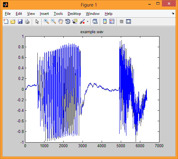


The first illustration shows the language signal of example.wav, Discretized at 16 KHz and 16 bits.
In the second illustration, we have one block (interval) of the specified speech signal with a duration of 25.6 ms. This block corresponds to 409 samples.
In the third illustration we see one speech signal block after processing it with a first-order filter.
The fourth model shows us one block after applying the Hamming window.
The fifth illustration gives us 512 amplitude values of the fast Fourier transform of this single block.
Since these amplitude values of the fast Fourier transform coincide in pairs (for the corresponding complex values of the fast Fourier transform are pairwise complex conjugate), it is possible to take only 256 first amplitude values. These 256 amplitude values are reflected in the sixth illustration.
The seventh illustration gives the value of a 24-element vector, the components of which are obtained after averaging 256 amplitude values within 24 “triangular” frequency bands.
Source: https://habr.com/ru/post/159605/
All Articles