The competition “Internet Mathematics: Yandex.Maps” - the experience of our participation and the description of the winning algorithm
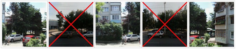
More than a year has passed since the end of the competition " Internet Mathematics: Yandex.Maps ", but we are still being asked about the algorithm that brought us victory in this competition. Having learned that Yandex recently announced the launch of the next " Internet Mathematics ", we decided to share the experience of our last year’s participation and describe our approach. The developed algorithm was able with an accuracy of 99.44% to correctly identify unnecessary images in a series of panoramic images, for example, like this:
In this article, we describe the basic ideas of the algorithm and provide details for those interested in it, talk about the lessons learned and how it all was.
')
The source code of our solution is available on github (C ++ using OpenCV ).
In 2011, Yandex offered the contestants an interesting task on computer vision, so our company specializing in this area would be a sin not to take part. The task was to search for unnecessary images in a series of panoramic images with Yandex.Maps. In each series 5 images were given, some of which (3, 4 or all 5) were made in one place and approximately at the same time, and the rest were superfluous. For example, images 1, 3 and 5 in the series above constitute a panorama, and images 2 and4 are superfluous . A total of 6000 episodes were given and it was required to find extra shots in each of them.
Having learned about the competition from our corporate newsletter, each of us downloaded data for ourselves, stubbornly looked at the pictures for several days (there was somethingto do - there were only 6000 x 5 pictures = 30,000) and hoped to win alone. It soon became clear that the task was actually not as simple as it seemed at first glance. Therefore, we decided to get together, discuss ideas and hold talks on a possible joint effort. As it turned out, we had very different approaches to solving the problem and it would be great to complement each other in the same team. So we did, and then everything follows the standard scheme: we created a common code repository, wrote an infrastructure for testing the accuracy of algorithms, and each set about working out his own ideas. We studied suitable articles, periodically brainstormed, tried new ideas and discarded broken ones ... So a month went by.
And then came the finalday - according to the terms of the competition, on the last day, Yandex gave out a new data set, on which it was necessary to drive the algorithm and get an answer in 24 hours. Our team was facing a sleepless night at work, so the first priority was the purchase of chips and all that was needed for productive programming. After gaining access to the final data set, we launched the best version of our algorithm, looked at a new batch of 30,000 images and until the last generated new ideas to take into account new data properties (though by 5 am some kind of nonsense was obtained, which until now then we have a reason for joking). Everything turned out to be not in vain: in a few days we learned that our team “Mythical Nizhny Novgorod” became the winner of the competition!
Next, we will talk about what algorithm we have in the end.
So, the task is to divide a series of images into groups: the desired panorama and superfluous images. To find such a partition, it is necessary for any pair of images to be able to assess the plausibility of the fact that they belong to the same panorama. To do this, we introduced two measures of similarity for a pair of images based on complementary approaches: a comparison of color histograms of images and the search for common parts in images. We combined these two measures into one and used the obtained measure to divide images into groups (clustering). The measure of each approach could be used separately, but the combination allows you to combine their strengths.
Histograms allow you to compare the frequency of occurrence of colors on one image with frequencies on the other. Since, according to the description of the task, the pictures in one panorama depict one scene at the same time from close camera positions, their color characteristics are usually similar to each other, and in extra pictures they are usually different. Therefore, the distance between the histograms gives a suitable estimate of the proximity of the images. For example, superfluous images from the series given at the beginning of the article are much darker than panoramic images, therefore dark colors will dominate in the histograms of extra images, and these histograms will be far from the panoramic image histograms.
The second approach, the search for common parts in the images, makes it possible to determine that two images belong to the same panorama in the case when there is a sufficient intersection between them, for example, the same object is found on them. This is achieved by using a popular approach in computer vision: the two key images are compared to the characteristic key points, after which a search is made for correspondences between them, for example, by comparing the neighborhoods of these points. If you managed to find many similar neighborhoods, then most likely they refer to the same objects and these are two images of the same scene. In this approach, the measure of proximity is the number of similar neighborhoods. For example, the work of this approach is illustrated in Fig. 1 and 2.
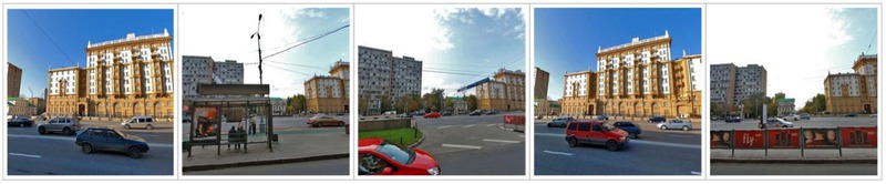
Fig. 1. An example of a series in which the search for common parts gives the correct classification, since the photographs contain parts of the same building. At the same time, color histograms of images 1 and 4 are very different from the others, therefore the histogram approach considers these two images as superfluous, which is in fact incorrect.

Fig. 2. Corresponding key points found by the algorithm.
These two approaches complement each other. The histogram approach can work even when there are no intersections and common parts between images of the same panorama (see the example in Fig. 3). However, in some cases there is an intersection between the images, but the other parts are very different in color (for example, the sun went down behind a cloud). In this case, the histograms will be far from each other, and the search for common parts can determine that these images still belong to the same panorama even by a small overlap (see the example in Fig. 1 and 2).
Fig. 3. An example of a series in which between images of one panorama (3, 4 and 5) there are no areas with common key points, but thanks to the color histograms, the correct classification is obtained (images 1 and2 are redundant ).
Experiments have shown that most of the correct answers can give a histogram approach alone, and the addition of the second approach only improves the classification in a few cases.
For those interested in computer vision and details of these two approaches, the following two sections are written, and all others are invited to proceed to the Combination of two approaches and Results .
During the implementation, the color space YCrCb was used, since it explicitly highlighted the brightness component. This allows you to take a smaller number of bins (grouping intervals) for this component and thereby increase the stability of the algorithm to changes in light and shadows.
We also added anotherone to these three components (Y, Cr, Cb) for constructing histograms - the ordinate of the pixel in the image to take into account the spatial arrangement of colors. This idea allows you to more accurately compare the colors of objects that are usually located at the same height: the road should be compared with the road, grass with grass, sky with sky. Such splitting of the image into horizontal stripes was introduced due to the fact that in the contest data the images within one panorama are shifted relative to each other mainly horizontally.
Thus, a four-dimensional histogram was constructed with 12 bins for brightness, 256 bins for each of the two color components and 4 bins for the pixel ordinate.
To calculate the distance between histograms, their intersection distance was used ( Histogram Intersection Distance ). For single-resolution images, this distance actually reflects the number of similar pixels between two images.
One of the most successful methods in computer vision is the use of unique local features in the image, such as angles or blob centers (small homogeneous areas). This approach is applicable if the scene is rather textural, that is, it contains a large number of such local features. The images from Yandex.Maps depict textural street scenes, so this approach is reasonable to use. However, there are several difficulties in the competitive data set: images have a low resolution (300x300 pixels) and there are often large non-textural areas (asphalt, sky, ...). Such low resolution results in low repeatability of the detector of local features: the key point found in one of the images will often not be detected in another image of the same panorama, and we will not be able to determine that there are matches between the images. To solve these problems, we set up such parameters of the detector of local features so that it finds a large number of key points in the image (~ 10k). However, this leads to the fact that the features on the compared images become less unique, and false matches are often found when searching for corresponding features. Therefore, we applied several additional filterings to select the correct matches. We turn to the details.
In many images, this algorithm lacked even a small intersection between images in order to find a sufficient number of corresponding key points. So, an interesting and unexpected example of the operation of the described algorithm is shown in Fig. four.
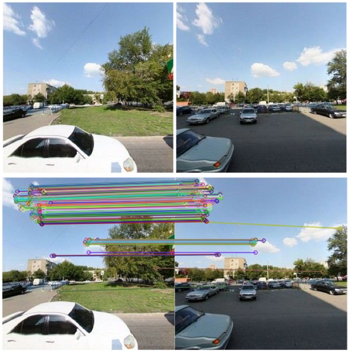
Fig. 4. An amusing situation when pictures can be combined into one panorama by the presence of the same clouds in the sky. In this pair of histogram snapshots, they feel insecure because of the large shadow, but local features and cloudy weather save the situation.
The described approaches allow calculating two types of distances between images. To take both approaches into account, we combine these distances as follows:
d comb = min ( c * d hist , d feat ),
Where
d comb - combined distance
d hist and d feat are the distances normalized to the interval [0, 1], calculated using the approaches on the histograms and local features, respectively;
c - coefficient less than one, which allows to give greater priority to the results of the algorithm that uses histograms.
To combine the two approaches, the minimum function was chosen, because if at least one of the two distances is small, then the images are really close.
Having calculated pairwise combined distances between images of one series, we perform hierarchical clustering ( Agglomerative hierarchical clustering using single-linkage ) of these images. The cluster with the maximum number of elements is recognized as the desired panorama, and the remaining images are superfluous. Such hierarchical clustering is very natural for this task, since within one panorama there may be distant non-intersecting images that are connected by a chain of other panorama images that are close to each other, and this method allows you to combine such images into one panorama.
So, after working hard on our algorithm, he showed a very good result on the final data set: 99.44% of images were correctly classified, which allowed to take first place in the competition. And also get a prize in the amount of 100,000 rubles to celebrate the victory :-)
As a conclusion, we want to share a few lessons that we have learned or consolidated by participating in the competition. They are definitely useful to us.
See you at the next contests on computer vision!
The authors of the article:
Maria Dimashova (Itseez, research engineer), mdim
Ilya Lysenkov (Itseez, research engineer), billys
In this article, we describe the basic ideas of the algorithm and provide details for those interested in it, talk about the lessons learned and how it all was.
')
The source code of our solution is available on github (C ++ using OpenCV ).
Description of the competitive task
In 2011, Yandex offered the contestants an interesting task on computer vision, so our company specializing in this area would be a sin not to take part. The task was to search for unnecessary images in a series of panoramic images with Yandex.Maps. In each series 5 images were given, some of which (3, 4 or all 5) were made in one place and approximately at the same time, and the rest were superfluous. For example, images 1, 3 and 5 in the series above constitute a panorama, and images 2 and
From start to finish
Having learned about the competition from our corporate newsletter, each of us downloaded data for ourselves, stubbornly looked at the pictures for several days (there was something
And then came the final
Next, we will talk about what algorithm we have in the end.
The basic ideas of the algorithm
So, the task is to divide a series of images into groups: the desired panorama and superfluous images. To find such a partition, it is necessary for any pair of images to be able to assess the plausibility of the fact that they belong to the same panorama. To do this, we introduced two measures of similarity for a pair of images based on complementary approaches: a comparison of color histograms of images and the search for common parts in images. We combined these two measures into one and used the obtained measure to divide images into groups (clustering). The measure of each approach could be used separately, but the combination allows you to combine their strengths.
Histograms allow you to compare the frequency of occurrence of colors on one image with frequencies on the other. Since, according to the description of the task, the pictures in one panorama depict one scene at the same time from close camera positions, their color characteristics are usually similar to each other, and in extra pictures they are usually different. Therefore, the distance between the histograms gives a suitable estimate of the proximity of the images. For example, superfluous images from the series given at the beginning of the article are much darker than panoramic images, therefore dark colors will dominate in the histograms of extra images, and these histograms will be far from the panoramic image histograms.
The second approach, the search for common parts in the images, makes it possible to determine that two images belong to the same panorama in the case when there is a sufficient intersection between them, for example, the same object is found on them. This is achieved by using a popular approach in computer vision: the two key images are compared to the characteristic key points, after which a search is made for correspondences between them, for example, by comparing the neighborhoods of these points. If you managed to find many similar neighborhoods, then most likely they refer to the same objects and these are two images of the same scene. In this approach, the measure of proximity is the number of similar neighborhoods. For example, the work of this approach is illustrated in Fig. 1 and 2.
Fig. 1. An example of a series in which the search for common parts gives the correct classification, since the photographs contain parts of the same building. At the same time, color histograms of images 1 and 4 are very different from the others, therefore the histogram approach considers these two images as superfluous, which is in fact incorrect.
Fig. 2. Corresponding key points found by the algorithm.
These two approaches complement each other. The histogram approach can work even when there are no intersections and common parts between images of the same panorama (see the example in Fig. 3). However, in some cases there is an intersection between the images, but the other parts are very different in color (for example, the sun went down behind a cloud). In this case, the histograms will be far from each other, and the search for common parts can determine that these images still belong to the same panorama even by a small overlap (see the example in Fig. 1 and 2).
Fig. 3. An example of a series in which between images of one panorama (3, 4 and 5) there are no areas with common key points, but thanks to the color histograms, the correct classification is obtained (images 1 and
Experiments have shown that most of the correct answers can give a histogram approach alone, and the addition of the second approach only improves the classification in a few cases.
For those interested in computer vision and details of these two approaches, the following two sections are written, and all others are invited to proceed to the Combination of two approaches and Results .
Details of the histogram approach
During the implementation, the color space YCrCb was used, since it explicitly highlighted the brightness component. This allows you to take a smaller number of bins (grouping intervals) for this component and thereby increase the stability of the algorithm to changes in light and shadows.
We also added another
Thus, a four-dimensional histogram was constructed with 12 bins for brightness, 256 bins for each of the two color components and 4 bins for the pixel ordinate.
To calculate the distance between histograms, their intersection distance was used ( Histogram Intersection Distance ). For single-resolution images, this distance actually reflects the number of similar pixels between two images.
Details of the approach based on local features
One of the most successful methods in computer vision is the use of unique local features in the image, such as angles or blob centers (small homogeneous areas). This approach is applicable if the scene is rather textural, that is, it contains a large number of such local features. The images from Yandex.Maps depict textural street scenes, so this approach is reasonable to use. However, there are several difficulties in the competitive data set: images have a low resolution (300x300 pixels) and there are often large non-textural areas (asphalt, sky, ...). Such low resolution results in low repeatability of the detector of local features: the key point found in one of the images will often not be detected in another image of the same panorama, and we will not be able to determine that there are matches between the images. To solve these problems, we set up such parameters of the detector of local features so that it finds a large number of key points in the image (~ 10k). However, this leads to the fact that the features on the compared images become less unique, and false matches are often found when searching for corresponding features. Therefore, we applied several additional filterings to select the correct matches. We turn to the details.
- As a detector of local features, we used FAST , which allows you to quickly find angles in the image. For the stability of the algorithm to change the distance to the objects to be shot at different camera positions, it is necessary to detect local features of different scales. To do this, we scale the images using 4 levels of the Gaussian pyramid of images , launch FAST at each level and combine the sets of found key points.
- For the key points of each image, we calculate the descriptors (descriptors) of their neighborhoods. We used the SURF descriptor, which is faster than the more well-known SIFT , but has a comparable quality.
- Next, we find the corresponding key points in the two images, using the calculated descriptors, which are 64-dimensional vectors of real numbers. For this purpose, for each descriptor of one image, the nearest descriptor is located in another image along the L1 distance between the descriptor vectors. This distance is more resistant to noise than the standard Euclidean distance. Since we have a huge number of local features, searching the nearest descriptor by brute force would take too much time. Therefore, we used an approximate search for the nearest descriptor using the FLANN library integrated into OpenCV.
- Found matches between local features are filtered by the criterion of cross-check reliability, which of all matches leaves only one-to-one.
- We filter the remaining matches by the y coordinate: if the y coordinates of the points connected by a match differ by more than 100 pixels (the parameter value is chosen experimentally), then we consider such a match to be false. This filter is based on the fact that only horizontal panoramas were found in the competitive images.
- We calculate the homology matrix according to the RANSAC scheme using a set of one-to-one correspondences between local singularities. According to the theory , between the points of the images there is a homography transformation (with an arbitrary change in the position of the camera), if their prototypes in the 3D world lie on the same plane. For non-planar objects, we can also search for a homography transformation, if the deviation of the object points from the flat shape is much smaller than the distance from the camera to the object. The search for homography for competitive images of panoramas is justified by the following facts: 1) the presence of planes is characteristic of objects of urban scenes; 2) objects are often sufficiently removed to be considered flat; 3) the computation of homography requires fewer iterations of the RANSAC than is necessary to find the fundamental matrix .
In the RANSAC homography search cycle, several heuristics were used to assess the quality of the next homography hypothesis: filter on the minimum singular number of the homography matrix, filter inlayers (matches that satisfy the current hypothesis on the homography matrix) for consistency of changes in orientations of the detected angles, replacing closely spaced inlays with one . As a result, the homography was chosen, which gives the largest number of inlays. - As a measure of proximity between images, the number of inlays for the found homography matrix is taken.
In many images, this algorithm lacked even a small intersection between images in order to find a sufficient number of corresponding key points. So, an interesting and unexpected example of the operation of the described algorithm is shown in Fig. four.
Fig. 4. An amusing situation when pictures can be combined into one panorama by the presence of the same clouds in the sky. In this pair of histogram snapshots, they feel insecure because of the large shadow, but local features and cloudy weather save the situation.
Combining two approaches
The described approaches allow calculating two types of distances between images. To take both approaches into account, we combine these distances as follows:
d comb = min ( c * d hist , d feat ),
Where
d comb - combined distance
d hist and d feat are the distances normalized to the interval [0, 1], calculated using the approaches on the histograms and local features, respectively;
c - coefficient less than one, which allows to give greater priority to the results of the algorithm that uses histograms.
To combine the two approaches, the minimum function was chosen, because if at least one of the two distances is small, then the images are really close.
Having calculated pairwise combined distances between images of one series, we perform hierarchical clustering ( Agglomerative hierarchical clustering using single-linkage ) of these images. The cluster with the maximum number of elements is recognized as the desired panorama, and the remaining images are superfluous. Such hierarchical clustering is very natural for this task, since within one panorama there may be distant non-intersecting images that are connected by a chain of other panorama images that are close to each other, and this method allows you to combine such images into one panorama.
results
So, after working hard on our algorithm, he showed a very good result on the final data set: 99.44% of images were correctly classified, which allowed to take first place in the competition. And also get a prize in the amount of 100,000 rubles to celebrate the victory :-)
Contest Lessons
As a conclusion, we want to share a few lessons that we have learned or consolidated by participating in the competition. They are definitely useful to us.
- Without friends I have a little bit, but with friends there are many. Participating as a team was our best decision ever. None of us could have won the competition alone. Together we generated ideas, were able to test many different approaches in parallel, used everyone’s knowledge and experience, supported and inspired each other and did not let anyone fall asleep on the last night before the deadline, continuing to generate delusions at 5 am. And the victory is more pleasant to celebrate all together.
- Woe from mind (or overfitting). At the beginning of the competition, Yandex provided marked data for preliminary testing of algorithms. However, in many series it was almost impossible to find the extra images even to a person (see the example in Fig. 5).
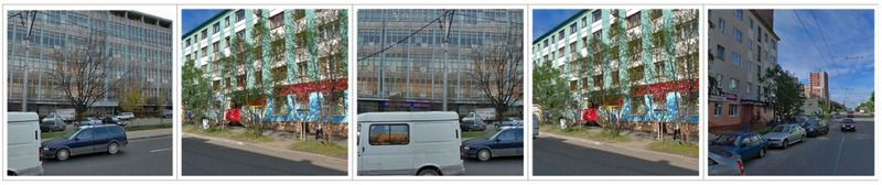
Fig. 5. An example of a very difficult series. What do you think, what images are superfluous?Answer1 and 3 are superfluous images, and 2, 4 and 5 form one panorama. If you look closely, then extra shots were taken at other times of the year.
The problem with the unsolvable series was raised by the participants at the contest forum, and the organizers promised not to allow this in the final data set. This meant that the final data set would have other properties than the preliminary set. Thus, the fundamental assumption of machine learning algorithms that the training and test sample should be generated by a single probability distribution was not fulfilled. Therefore, we decided to use the simplest algorithms with a small number of adjustable parameters, since otherwise the risk of retraining is extremely high. As practice has shown, this was a very valuable observation, since several other participants using advanced machine learning algorithms really retrained and showed not such a good result on the final data as on the preliminary ones. - Behold the root. To test ideas, understand the behavior and problems of algorithms, and just debug, you need the correct visualization (of both the final results and intermediate steps). This allowed us to feel the specifics of the problem and the data, to move more clearly and quickly to the right solutions.
- Small, yes removed. The solution of the problem is to start with simple approaches: they are very easy and quick to implement, but the result will be immediately obtained for comparison (baseline). Moreover, even a primitive approach can show surprisingly good results, and if you do a little bit of it for the specifics of the task, then it can become invincible. This is what happened to us with histograms: a very simple idea that brought us the main result (local features increased the classification accuracy by less than one percent). In this case, the calculation of all the final data by histograms took only a couple of minutes, and we waited several hours for the results of the approach on local features.
- Right hook, left hook. Attacking a task is better from different angles: it is useful to develop alternate problem solving strategies and have the tools that can cope with all the discovered properties of the task. For example, we tried approaches that take into account color, gradients and their orientations, spatial position, absence and the presence of overlaps between images. As a result, to improve the accuracy of classification, we combined the solutions found.
- Don't worry, be happy. We did not forget to enjoy the process, appreciated the opportunity to learn something new and communicate with each other. It was a very pleasant and rewarding experience. Winning a
competition is , of course, great, but we often remember not the moment of the announcement of results, but many other funny and crazy moments during the time of participation in thecompetition - this is for life :-)
See you at the next contests on computer vision!
Useful materials on Habré
- Algorithm of another team: Solving the problem “Yandex Internet Mathematics - 2011”. Definition of visual similarity of images
- Detector and SURF Descriptor Description: Detecting Persistent Image Characteristics : SURF Method
- Detector and SIFT Descriptor Description: Building SIFT Descriptors and Image Matching Task
- Description of an alternative approach to filtering matches: Filtering false matches between images using a dynamic matching graph
- Tutorial about the standard scheme for applying local features (detector + handle + matching search + homography): OpenCV 2.4 flat object recognition
The authors of the article:
Maria Dimashova (Itseez, research engineer), mdim
Ilya Lysenkov (Itseez, research engineer), billys
Source: https://habr.com/ru/post/158645/
All Articles