Talmud formulas in Google SpreadSheet
Usually we write about hosting, in particular, about foreign shared hosting in the United States. But to write, you need to have analytical data at hand . This is where Google Docs help is required if the file is supposedly less than 400,000 lines.
For several months of working with tables, Google had to analyze many times using formulas of various kinds of data . As expected - what could be solved in MS Excel can be implemented in Google spreadsheets. But numerous attempts to solve problems with the help of a favorite search engine led only to new questions and almost to zero answers.
Therefore, it was decided to make life easier for others and glorify themselves .
In order for Excel or spreadsheet (Google table) to understand that what is written is a formula, you need to put an "=" sign in the formula bar (Figure 1).
Picture 1
Next, we begin to write the formula from the keyboard or select the cells with which we are going to work with the mouse.
To determine the cell can be used 2 types of symbols:
Cell address “B3” in such a system will look like R3C2 (R = row = row, C = column = column). For scripts, for example, both styles are used.
Where we write "= formula", for example, = SUM (A1: A10) and our value will be displayed.
The general principle of operation of RC formulas is shown in Figure 2.
')
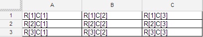
Figure 2
As can be seen from Figure 3, the values of the cells are relative to the cell in which the formula with the equal sign will be written. To preserve the aesthetic appearance of the formulas, the characters [0] are written in them, which you may not have to write: R [0] C [1] = RC [1].
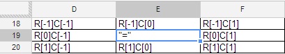
Figure 3
The difference between Figure 2 and Figure 3 is that Figure 3 is a universal formulation that is not tied to rows and columns (look at the values of rows and columns), which cannot be said about Figure 2. But the RC style in the spreadsheet is mainly used for writing javascript scripts.
For accessing cells, links are used that come in 3 types:
The $ sign here indicates the type of link. Differences between different types of links can be seen by pulling the autocomplete marker of the active cell or range of cells containing a formula with links.
The relative link “remembers” at what distance (in rows and columns) you clicked RELATIVE to the position of the cell where you put “=” (offset in rows and columns). Then pull down the autocomplete marker, and this formula will be copied to all the cells through which we stretched.
As mentioned above, if you pull the formula containing relative links for the auto-complete marker, the table will recalculate their addresses. If the formula contains absolute links, their address will remain unchanged. Simply put - an absolute link always point to the same cell.
To make the relative reference absolute, it is enough to put the “$” sign in front of the letter of the column and the address of the line, for example, $ A $ 1. A quicker way is to select a relative link and press the “F4” key once, while the spreadsheet itself will put down the “$” sign. If you press "F4" a second time, the link will become mixed type A $ 1, if the third time is $ A1, if it is the fourth time, the link will become relative again. And so in a circle.
Mixed links are half absolute and half relative. The dollar sign in them is either before the letter of the column or before the row number. This is the most difficult to understand link type. For example, the cell contains the formula “= A $ 1”. Reference A $ 1 is relative in column A and absolute in line 1. If we pull this formula up or down for the auto-fill marker, then the links in all copied formulas will point to cell A1, that is, they will behave as absolute. However, if we pull right or left, the links behave as relative, that is, the spreadsheet will begin to recalculate its address. Thus, formulas created by auto-completion will use the same line number ($ 1), but the literal value of the column will change (A, B, C ...).
Let's look at an example of summing up cells with multiplication by a certain coefficient.
This example assumes the presence of a coefficient value in each calculated cell (cells D8, D9, D10 ... E8, F8 ...). (Figure 4).
The red arrows indicate the direction of stretching with a marker filling the formula that is in cells C2. In the formula, notice the change in cell D8. When stretching downwards, only the number symbolizing the string changes. When stretching to the right, only the column changes.

Figure 4
Simplify the example by applying the $ sign (Figure 5).
Figure 5
But it is not always necessary to freeze all the columns and rows, sometimes only a row or a column is used. (Figure 6)
Figure 6
All formulas can be read on the official site support.google.com
Important: The data that must be processed in the formulas should not be in different documents, it is possible to do this only with the help of scripts.
If you write the formula incorrectly, a comment about the syntax error in the formula will inform you about it (Figure 7).

Figure 7
Although errors can be not only syntactic, but also, for example, mathematical, such as division by 0 (Figure 7) and others (Figure 7.1, 7.2, 7.3). To see a note that shows what error occurred, move the cursor over the red triangle in the upper right corner of the error.

Figure 7.1
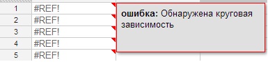
Figure 7.2
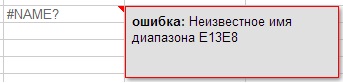
Figure 7.3
For the convenience of perception of the table, all cells with formulas will be painted in purple.
To see the formulas “live”, press the Ctrl + hot key or select (View)> All formulas from the menu above. (Figure 8).

Figure 8
In the formulation of formulas in the directory and in the formulas that are used to work at the moment, there are differences. They consist in the fact that instead of the “comma”, which was used earlier in many formulas, the “semicolon” is already used (the changes occurred more than six months ago).
In order to see what the formula refers to on this page (Figure 9), you need to click the mouse in the formula bar to the right of the Fx inscription (Fx is located below the main menu on the left).
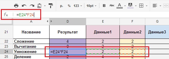
Figure 9
IMPORTANT: For the correct functioning of the formulas, they must be written in LATIN letters. Russian (Cyrillic) “A” or “C” and Latin “A” or “C” for a formula are 2 different letters.
To paint, of course, the eternal operations of addition, subtraction, etc., no one will, but they will help you understand the basics. With a few examples, you will understand how they work in this environment. In the document, the link to which is given at the end of the article, all the formulas are given, we just stop at the screenshots.
We have the initial data in the range E22: H25, and the result in column D. Figure 10 shows the header for all the data that will be used.
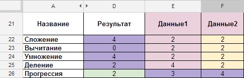
Figure 10
Recall that if you want to use a range, it will summarize all the cells in a row, and if you need to sum the cells in a specific order, then they must be specified with “;” in the correct order. We have the initial data for the progression in cell D26, and the result in cells E26: H26 (Figure 11) Used to number the rows and columns.

Figure 11
We have the initial data in cell E28, and the result in cell D28 (Figure 12)

Figure 12
ROUND rounds off according to mathematical laws, if after a comma there is a digit 5 or more, the integer part is increased by one, if 4 or less, it remains unchanged, also rounding can be done using the FORMAT menu -> Numbers -> “1000, 12 ”2 decimal places (Figure 13). If you need more characters, then you need to press FORMAT -> Numbers -> Personalized decimal -> And specify the number of characters.
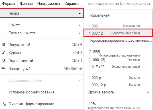
Figure 13
Probably the most familiar feature.
We have the initial data in cells E30 and H30, and the result in cell D30

(Figure 14).
The amount if the cells go in sequence.

Figure 15
We have the initial data in the range of cells E32: H32, and the result in cell D32 (Figure 16).

Figure 16
Of course, there are others, but we go further.
From the great number of textual formulas, with the help of which you can do anything with the text, the most demanded one, in my opinion, is the formula for “gluing” text values. There are several options for its execution:
We have the initial data in the range of cells E36: H36, and the result in cell D36 (Figure 17).
Using Google documents, employees often conduct employee surveys or compile polls via Google Forms (these are special forms that can be created via the Insert-> Form menu. After filling out the form, the data are presented in a table. And then, use different formulas for working with data, for example , for pasting full name).
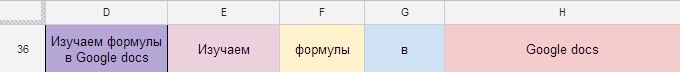
Figure 17
We have the initial data in the range of cells E37: H37, and the result in cell D36 (Figure 18 - glued numbers).
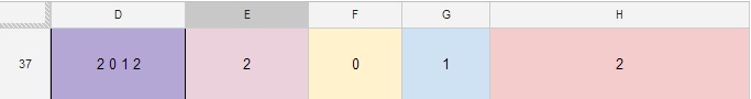
Figure 18
We have the initial data “1 more”, “uses”, “as NAM” and in the range of cells E38: G38, therefore it is advisable to use this type of formula, and the result in cell D36 (Figure 19).
Glue the text and numeric values.
Figure 19
We come to the most interesting, in my opinion, functions: LOGICAL AND OTHER.
One of the most necessary formulas:
We have the initial data on the Data sheet, cell A15 (Figure 20), and the result on the Formula sheet in cell D41 (Figure 20.1).
Figure 20

Figure 20.1
Most of the programs for working with tables contain two types of array formulas: “for several cells” and “for one cell”.
Google spreadsheets divide these types into two functions: CONTINUE (CONTINUE) and ARRAYFORMULA.
Array formulas for multiple cells allow the formula to return multiple values. You can use them, even without knowing it, simply by entering a formula that returns several values.
Array formulas “in one cell” allow you to write formulas using array input, rather than output data. When entering a formula into the function = ARRAYFORMULA, you can pass arrays or ranges to functions and operators, which, as a rule, use only arguments that do not belong to arrays. These functions and operators will be applied one by one for each record in the array, and return a new array with all the output data.
If you want to explore the issue in more detail, you should visit support.google .
In simple words, to work with formulas that return arrays of data, in order to avoid syntactical errors, it is necessary to enclose them in an array of formulas.
In order to operate with logical formulas, and they usually contain large data arrays, they are placed into an array of formulas ARRAYFORMULA (formula).
For an explanation of the formula, let us analyze an example in detail: the 3rd buyers were instructed to buy products according to the list, but pay in one amount. After the products were punched at the checkout, the list of products (Figure 21) in column A was obtained, and their number in column B.
The task, what kind of fiscal receipt will have after printing (you just need to fold the products of 3 buyers and find out the number of products in the amount for each position)?
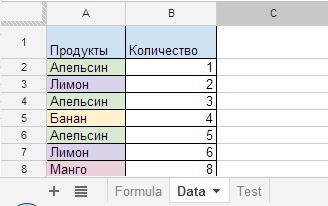
Figure 21
We have the initial data in the Data sheet (Figure 21), and the result on the Formula sheet in column D (Figure 22). In columns E, F, G, the arguments used in the formula are shown, and in column H, the general form of the formula that is in column D and calculates the result.
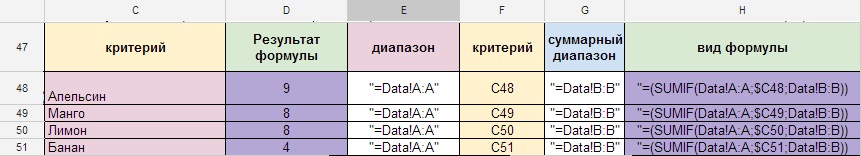
Figure 22
The example above shows a general view of the operation of the “Sum If” formula with one condition, but the “IF Amount” (with many conditions) is most often used.
We continue to consider the problem with the products on another level.
The party is just beginning, and after the call of friends, you begin to understand that there is not enough alcohol. And you need to buy it. Each friend should bring a hot drink. You need to know the number of bottles of beer that you want to bring, and give the task to your friends.
We have the initial data on the Data sheet (Figure 23).
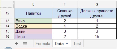
Figure 23
Suppose that on the Formula sheet, in cell B53 (criterion_1 = Beer) there should be the name of the drink, and cell C53 (criterion_2 = 2) is the number of friends who will bring Beer. As a result, in the D53 cell, the result will be that we need to purchase 15 bottles of beer. (Figure 23.1) that is, the formula will determine the amount of two criteria - beer and the number of friends.
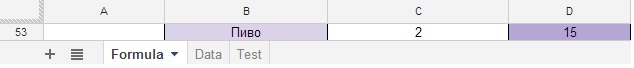
Figure 23.1
If there are more such positions, lines 16 and 21 (Figure 24), then the number of bubbles in column G is summed (Figure 24.1).
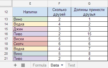
Figure 24
Total:
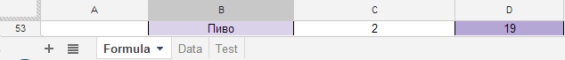
Figure 24.1
Ha ... the party goes on, and you remember that you need a cake, but not an easy one, but a super one - a mega cake, with different spices, which, unfortunately, are also encrypted under digital symbols. The challenge is to buy spices in the right amount of bags of each of the spices. The chef encrypted the required amount into a table (Figure 25.1), columns A and B (in the adjacent columns we do our calculations).
Each spice has its own serial number: 1,2,3,4. (Figure 25).
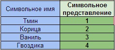
Figure 25
Our task is to count the number of duplicate values, in our case, these are numbers from 1 to 4 in column B and determine how many percent fall on each of the spices.
We have the initial data in the range A55: B61, the selection condition is selected by cell F55 and E59: E62, and the result is in the cell range F59: F62 (counting the number of repetitions of numerical values when the conditions coincide).

Figure 25.1
In the end, we have the amount of repetitions and the percentage.
To correctly write a formula, you must fully understand what you HAVE, WHAT YOU WANT TO GET, and in what form. Perhaps for this you have to change the appearance of the initial data.
Go to the next example.
If the formulas use values in “merged cells”, then the first cell for the merged data is indicated, in our case it is column F, and cell F65 (Figure 26)
Figure 26.
Finally, we got to the worst formulas.
There are several types of such calculations, they are suitable for large tables in which you need to count the number of identical words or the number of numbers. But with the correct understanding of these formulas, it is possible to perform such miracles with them as, for example: counting words without taking into account the words of exceptions. Examples below.
We have the initial data in the range of cells E70: H70, and the result in cell D70 (Figure 27 - counting cells containing numerical values in the range in which there are cells with text).
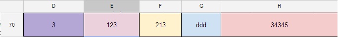
Figure 27.
Cells containing text and numbers are also not counted.
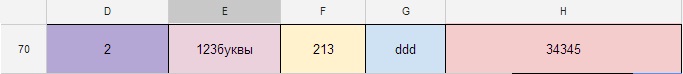
Figure 27.1.
We have the initial data in the range of cells E71: H71, and the result in cell D71 (Figure 28 - the counting of all values in the range).
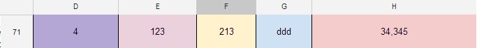
Figure 28.
Also, the formula considers cells that contain only punctuation marks, tabs, but does not count empty cells.
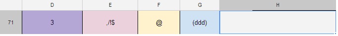
Figure 28.1
We have the initial data in cells F73 and H73, and the result in cell D73 (If F73 = 5 and H73 = 5, then D73 = 0 in all other cases 1) (Figure 29).

Figure 29.

Figure 29.1
Let's complicate the example.
Count the number of cells in which time frames are written without taking into account the words “auto answer”, “busy”, “-”.
We have the initial data in the range of cells E74: H75, and the result in cell D74 (Figure 30).
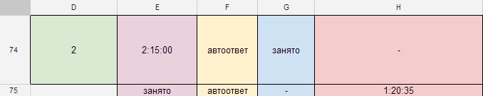
Figure 30
So we’ve come to the end of our little educational program using formulas in Google SpreadSheet and I have high hopes that I have shed light on some aspects of analytical work with formulas.
The formulas, to be honest, were literally suffered. Each of them was created over time. I hope you enjoyed my article and the examples in it.
And finally, as a gift. And forgive me, the developers!
If you need to hide the document from the eyes of others forever, then this formula is for you.
The formula itself: "= (ARRAYFORMULA (SUMIF ($ A: $ A & $ C: $ C; $ H: $ H & F $ 2; $ C: $ C)))". $ H: $ H governs the distribution of the formula. After fomlula run (Figure 31), below in the cells, it will begin to multiply the next function CONTINUE (cell; row; column).
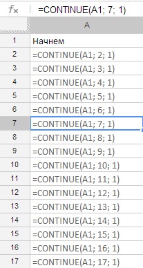
Figure 31
The formula cyclically adds formulas to the entire column. In order to kill a document, you need to try a little, create an N-th number of cells and write the formula in the first cells of the N-th number of columns. Everything! The document can no longer be corrected and verified!
This is what Google’s help page says about workload and restrictions - http://support.google.com/drive/bin/answer.py?hl=en&p=spreadsheets_timeout&answer=2505921 The
promised Talmud document was formulated as a basis in Google SpreadSheet .
Until new meetings, with respect Anton Piluganov.
For several months of working with tables, Google had to analyze many times using formulas of various kinds of data . As expected - what could be solved in MS Excel can be implemented in Google spreadsheets. But numerous attempts to solve problems with the help of a favorite search engine led only to new questions and almost to zero answers.
Therefore, it was decided to make life easier for others and glorify themselves .
Briefly about the main thing
In order for Excel or spreadsheet (Google table) to understand that what is written is a formula, you need to put an "=" sign in the formula bar (Figure 1).
Picture 1
Next, we begin to write the formula from the keyboard or select the cells with which we are going to work with the mouse.
To determine the cell can be used 2 types of symbols:
- alphanumeric (LETTER = COLUMN; DIGIT = LINE) such as "A1".
- style R1C1, in the system R1C1 and the rows and columns are denoted by numbers.
Cell address “B3” in such a system will look like R3C2 (R = row = row, C = column = column). For scripts, for example, both styles are used.
Where we write "= formula", for example, = SUM (A1: A10) and our value will be displayed.
The general principle of operation of RC formulas is shown in Figure 2.
')
Figure 2
As can be seen from Figure 3, the values of the cells are relative to the cell in which the formula with the equal sign will be written. To preserve the aesthetic appearance of the formulas, the characters [0] are written in them, which you may not have to write: R [0] C [1] = RC [1].
Figure 3
The difference between Figure 2 and Figure 3 is that Figure 3 is a universal formulation that is not tied to rows and columns (look at the values of rows and columns), which cannot be said about Figure 2. But the RC style in the spreadsheet is mainly used for writing javascript scripts.
Link types (addressing types)
For accessing cells, links are used that come in 3 types:
- Relative references (example, A1);
- Absolute links (example, $ A $ 1);
- Mixed links (for example, $ A1 or A $ 1, they are half relative, half absolute).
The $ sign here indicates the type of link. Differences between different types of links can be seen by pulling the autocomplete marker of the active cell or range of cells containing a formula with links.
Relative links
The relative link “remembers” at what distance (in rows and columns) you clicked RELATIVE to the position of the cell where you put “=” (offset in rows and columns). Then pull down the autocomplete marker, and this formula will be copied to all the cells through which we stretched.
Absolute links
As mentioned above, if you pull the formula containing relative links for the auto-complete marker, the table will recalculate their addresses. If the formula contains absolute links, their address will remain unchanged. Simply put - an absolute link always point to the same cell.
To make the relative reference absolute, it is enough to put the “$” sign in front of the letter of the column and the address of the line, for example, $ A $ 1. A quicker way is to select a relative link and press the “F4” key once, while the spreadsheet itself will put down the “$” sign. If you press "F4" a second time, the link will become mixed type A $ 1, if the third time is $ A1, if it is the fourth time, the link will become relative again. And so in a circle.
Mixed links
Mixed links are half absolute and half relative. The dollar sign in them is either before the letter of the column or before the row number. This is the most difficult to understand link type. For example, the cell contains the formula “= A $ 1”. Reference A $ 1 is relative in column A and absolute in line 1. If we pull this formula up or down for the auto-fill marker, then the links in all copied formulas will point to cell A1, that is, they will behave as absolute. However, if we pull right or left, the links behave as relative, that is, the spreadsheet will begin to recalculate its address. Thus, formulas created by auto-completion will use the same line number ($ 1), but the literal value of the column will change (A, B, C ...).
Let's look at an example of summing up cells with multiplication by a certain coefficient.
This example assumes the presence of a coefficient value in each calculated cell (cells D8, D9, D10 ... E8, F8 ...). (Figure 4).
The red arrows indicate the direction of stretching with a marker filling the formula that is in cells C2. In the formula, notice the change in cell D8. When stretching downwards, only the number symbolizing the string changes. When stretching to the right, only the column changes.
Figure 4
Simplify the example by applying the $ sign (Figure 5).
Figure 5
But it is not always necessary to freeze all the columns and rows, sometimes only a row or a column is used. (Figure 6)
Figure 6
All formulas can be read on the official site support.google.com
Important: The data that must be processed in the formulas should not be in different documents, it is possible to do this only with the help of scripts.
Formula Errors
If you write the formula incorrectly, a comment about the syntax error in the formula will inform you about it (Figure 7).
Figure 7
Although errors can be not only syntactic, but also, for example, mathematical, such as division by 0 (Figure 7) and others (Figure 7.1, 7.2, 7.3). To see a note that shows what error occurred, move the cursor over the red triangle in the upper right corner of the error.
Figure 7.1
Figure 7.2
Figure 7.3
For the convenience of perception of the table, all cells with formulas will be painted in purple.
To see the formulas “live”, press the Ctrl + hot key or select (View)> All formulas from the menu above. (Figure 8).
Figure 8
How to write formulas
In the formulation of formulas in the directory and in the formulas that are used to work at the moment, there are differences. They consist in the fact that instead of the “comma”, which was used earlier in many formulas, the “semicolon” is already used (the changes occurred more than six months ago).
In order to see what the formula refers to on this page (Figure 9), you need to click the mouse in the formula bar to the right of the Fx inscription (Fx is located below the main menu on the left).
Figure 9
IMPORTANT: For the correct functioning of the formulas, they must be written in LATIN letters. Russian (Cyrillic) “A” or “C” and Latin “A” or “C” for a formula are 2 different letters.
Formulas
Arithmetic formulas.
To paint, of course, the eternal operations of addition, subtraction, etc., no one will, but they will help you understand the basics. With a few examples, you will understand how they work in this environment. In the document, the link to which is given at the end of the article, all the formulas are given, we just stop at the screenshots.
Addition, subtraction, multiplication, division.
- Description: addition, subtraction, multiplication and division formulas.
- Type of the formula: “Cell_1 + Cell_2”, “Cell_1-Cell_2”, “Cell_1 * Cell_2”, “Cell_1 / Cell_2”
- The formula itself: = E22 + F22, = E23-F23, = E24 * F24, = E25 / F25.
We have the initial data in the range E22: H25, and the result in column D. Figure 10 shows the header for all the data that will be used.
Figure 10
Progression.
- Description: a formula for incrementing all subsequent cells by one (numbering rows and columns).
- Formula view: = Previous cell + 1.
- The formula itself: = D26 + 1
Recall that if you want to use a range, it will summarize all the cells in a row, and if you need to sum the cells in a specific order, then they must be specified with “;” in the correct order. We have the initial data for the progression in cell D26, and the result in cells E26: H26 (Figure 11) Used to number the rows and columns.
Figure 11
Rounding
- Description: A formula for rounding the number in a cell.
- Type of formula: = ROUND (cell with a number); counter (how many numbers should be rounded after the comma).
- The formula itself: = ROUND (E28; 2).
We have the initial data in cell E28, and the result in cell D28 (Figure 12)
Figure 12
ROUND rounds off according to mathematical laws, if after a comma there is a digit 5 or more, the integer part is increased by one, if 4 or less, it remains unchanged, also rounding can be done using the FORMAT menu -> Numbers -> “1000, 12 ”2 decimal places (Figure 13). If you need more characters, then you need to press FORMAT -> Numbers -> Personalized decimal -> And specify the number of characters.
Figure 13
The amount if the cells are not consecutive.
Probably the most familiar feature.
- Description: Summation of numbers that are in different cells.
- Type of formula: = SUM (number_1; number_2; ... number_30).
- The formula itself: "= SUM (E30; H30)" we write through ";" if different cells.
We have the initial data in cells E30 and H30, and the result in cell D30
(Figure 14).
The amount if the cells go in sequence.
- Description: Summation of numbers that follow each other (sequentially).
- Type of formula: = SUM (number_1: number_N).
- The formula itself: = SUM (E31: H31) "write through": "if it is a continuous range.
- We have the initial data in the range of cells E31: H31, and the result in cell D31 (Figure 15).
Figure 15
Average.
- Description: summarizes the range of numbers and divides by the number of cells in the range.
- Type of formula: = AVERAGE (cell with number or number_1; cell with number or number_2; ... cell with number or number_30).
- The formula itself: = AVERAGE (E32: H32)
We have the initial data in the range of cells E32: H32, and the result in cell D32 (Figure 16).
Figure 16
Of course, there are others, but we go further.
Textual formulas.
From the great number of textual formulas, with the help of which you can do anything with the text, the most demanded one, in my opinion, is the formula for “gluing” text values. There are several options for its execution:
Gluing text values (formula).
- Description: “Gluing” Text Values (Option A).
- Formula type: = CONCATENATE (cell with number / text or text_1; cell with number / text or text_2; ..., cell with number / text or text_30).
- The formula itself: = CONCATENATE (E36; F36; G36; H36).
We have the initial data in the range of cells E36: H36, and the result in cell D36 (Figure 17).
Using Google documents, employees often conduct employee surveys or compile polls via Google Forms (these are special forms that can be created via the Insert-> Form menu. After filling out the form, the data are presented in a table. And then, use different formulas for working with data, for example , for pasting full name).
Figure 17
Gluing numeric values.
- Description: “sticking” text values with hands, without using special functions (option B - manual writing a formula, any formula complexity.).
- Formula type: = cell with number / text 1 & "" & cell with number / text 2 & "" & cell with number / text 3 & "" & cell with number / text 4 ("" is a space, the & sign means gluing, all text values are written in quotes "").
- The formula itself: = E37 & "" & F37 & "" & G37 & "" & H37.
We have the initial data in the range of cells E37: H37, and the result in cell D36 (Figure 18 - glued numbers).
Figure 18
Gluing numeric and textual values.
- Description: “gluing” text values with hands, without using special functions (option C - mixed type, any formula complexity).
- Formula type: = "text_1" & cell_1 & "text_2" & cell_2 & "text_3" & cell_3
- Important: all text that will be written in “” will be unchanged for the formula.
- The formula itself: = "Another 1" & E38 & "using" & F38 & "as US" & G38.
We have the initial data “1 more”, “uses”, “as NAM” and in the range of cells E38: G38, therefore it is advisable to use this type of formula, and the result in cell D36 (Figure 19).
Glue the text and numeric values.
Figure 19
LOGICAL AND OTHER
Transfer data from any sheets of the same file.
We come to the most interesting, in my opinion, functions: LOGICAL AND OTHER.
One of the most necessary formulas:
- Description: transfer data from any sheets of the same file (for Excel, you can transfer both from a sheet of one book to another sheet of the same book and from a sheet of one book to a sheet of another book).
- Type of formula: = "Name_List"! cell_1
- The formula itself: = Data! A15 (Data is a sheet, A15 is a cell on that sheet).
We have the initial data on the Data sheet, cell A15 (Figure 20), and the result on the Formula sheet in cell D41 (Figure 20.1).
Figure 20
Figure 20.1
Array of formulas.
Most of the programs for working with tables contain two types of array formulas: “for several cells” and “for one cell”.
Google spreadsheets divide these types into two functions: CONTINUE (CONTINUE) and ARRAYFORMULA.
Array formulas for multiple cells allow the formula to return multiple values. You can use them, even without knowing it, simply by entering a formula that returns several values.
Array formulas “in one cell” allow you to write formulas using array input, rather than output data. When entering a formula into the function = ARRAYFORMULA, you can pass arrays or ranges to functions and operators, which, as a rule, use only arguments that do not belong to arrays. These functions and operators will be applied one by one for each record in the array, and return a new array with all the output data.
If you want to explore the issue in more detail, you should visit support.google .
In simple words, to work with formulas that return arrays of data, in order to avoid syntactical errors, it is necessary to enclose them in an array of formulas.
Summation of cells with the condition IF.
In order to operate with logical formulas, and they usually contain large data arrays, they are placed into an array of formulas ARRAYFORMULA (formula).
- Description: summarizes cells with an IF condition (SUMIF formula).
- Formula Type: = SUMIF ('Sheet'! Range; Criteria; 'Sheet'! Total_Range)
For an explanation of the formula, let us analyze an example in detail: the 3rd buyers were instructed to buy products according to the list, but pay in one amount. After the products were punched at the checkout, the list of products (Figure 21) in column A was obtained, and their number in column B.
The task, what kind of fiscal receipt will have after printing (you just need to fold the products of 3 buyers and find out the number of products in the amount for each position)?
Figure 21
We have the initial data in the Data sheet (Figure 21), and the result on the Formula sheet in column D (Figure 22). In columns E, F, G, the arguments used in the formula are shown, and in column H, the general form of the formula that is in column D and calculates the result.
Figure 22
The example above shows a general view of the operation of the “Sum If” formula with one condition, but the “IF Amount” (with many conditions) is most often used.
Summation of cells IF, set of conditions.
We continue to consider the problem with the products on another level.
The party is just beginning, and after the call of friends, you begin to understand that there is not enough alcohol. And you need to buy it. Each friend should bring a hot drink. You need to know the number of bottles of beer that you want to bring, and give the task to your friends.
- Description: Amount IF (with many conditions).
- Formula view: = SUMIF ('Data'! Range_1 & 'Data'! Range_2; criteria_1 & criterion_2; 'Data'! Total_range).
- The formula itself: = (ARRAYFORMULA (SUMIF ((Data! E: E & Data! F: F); (B53 & C53); Data! G: G)))
We have the initial data on the Data sheet (Figure 23).
Figure 23
Suppose that on the Formula sheet, in cell B53 (criterion_1 = Beer) there should be the name of the drink, and cell C53 (criterion_2 = 2) is the number of friends who will bring Beer. As a result, in the D53 cell, the result will be that we need to purchase 15 bottles of beer. (Figure 23.1) that is, the formula will determine the amount of two criteria - beer and the number of friends.
Figure 23.1
If there are more such positions, lines 16 and 21 (Figure 24), then the number of bubbles in column G is summed (Figure 24.1).
Figure 24
Total:
Figure 24.1
Now we give a more interesting example:
Ha ... the party goes on, and you remember that you need a cake, but not an easy one, but a super one - a mega cake, with different spices, which, unfortunately, are also encrypted under digital symbols. The challenge is to buy spices in the right amount of bags of each of the spices. The chef encrypted the required amount into a table (Figure 25.1), columns A and B (in the adjacent columns we do our calculations).
Each spice has its own serial number: 1,2,3,4. (Figure 25).
Figure 25
Our task is to count the number of duplicate values, in our case, these are numbers from 1 to 4 in column B and determine how many percent fall on each of the spices.
- Description: Count the number of identical digits in large arrays under additional conditions.
- Formula view: READ IF ('Formula'! Range_A55: A61 + 'Formula'! Range_B55: B61; ConditionA ”Spices” + ConditionB ”number from 1 to 4”; Sheet ”Formula '! Range_B55: B61) / ConditionB” number from 1 to 4 ")
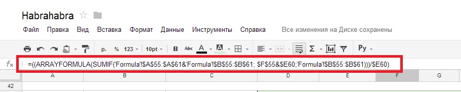
- The formula itself: = ((ARRAYFORMULA (SUMIF ('Formula'! $ A $ 55: $ A $ 61 & 'Formula'! $ B $ 55: $ B $ 61; $ F $ 55 & $ E59; 'Formula'! $ B $ 55: $ B $ 61))) / $ E59)
We have the initial data in the range A55: B61, the selection condition is selected by cell F55 and E59: E62, and the result is in the cell range F59: F62 (counting the number of repetitions of numerical values when the conditions coincide).
- Description: Calculates the percentage of spices.
- Type of formula: Amount * 100% / Total_number
- The formula itself: = F58 * $ G $ 56 / F $ 56
Figure 25.1
In the end, we have the amount of repetitions and the percentage.
To correctly write a formula, you must fully understand what you HAVE, WHAT YOU WANT TO GET, and in what form. Perhaps for this you have to change the appearance of the initial data.
Go to the next example.
Count the values in the merged cells.
If the formulas use values in “merged cells”, then the first cell for the merged data is indicated, in our case it is column F, and cell F65 (Figure 26)
- Description: A formula for counting values with the @ symbol.
- Formula view: READ IF (In column F of the “Formula” sheet there is text with the contents of @).
- The formula itself: = COUNTIF ('Formula'! F65: F68; "* @ *").
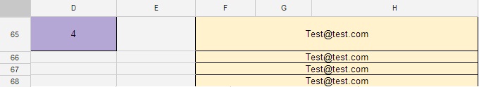
Figure 26.
Finally, we got to the worst formulas.
Counts the number of numbers in the argument list.
There are several types of such calculations, they are suitable for large tables in which you need to count the number of identical words or the number of numbers. But with the correct understanding of these formulas, it is possible to perform such miracles with them as, for example: counting words without taking into account the words of exceptions. Examples below.
- Description: Count the number of cells containing digits without text variables.
- Type of formula: COUNT (value_1; value_2; ... value_30)
- The formula itself: = COUNT (E45; F45; G45; H45)
We have the initial data in the range of cells E70: H70, and the result in cell D70 (Figure 27 - counting cells containing numerical values in the range in which there are cells with text).
Figure 27.
Cells containing text and numbers are also not counted.
Figure 27.1.
Counting the number of cells containing digits with text variables.
- Description: Count the number of cells containing digits with text variables.
- Type of formula: COUNTA (value_1; value_2; ... value_30)
- The formula itself: = COUNTA (E46: H46)
We have the initial data in the range of cells E71: H71, and the result in cell D71 (Figure 28 - the counting of all values in the range).
Figure 28.
Also, the formula considers cells that contain only punctuation marks, tabs, but does not count empty cells.
Figure 28.1
Substitution of values under conditions.
- Description: substitution of values under conditions.
- Formula: "= IF (AND ((Condition1); (Condition2)); The result is 0 if condition 1 and 2 is met; if not, the result is 1)"
- The formula itself: "= IF (AND ((F73 = 5); (H73 = 5)); 0; 1)"
We have the initial data in cells F73 and H73, and the result in cell D73 (If F73 = 5 and H73 = 5, then D73 = 0 in all other cases 1) (Figure 29).
Figure 29.
Figure 29.1
Let's complicate the example.
Count the number of cells in which time frames are written without taking into account the words “auto answer”, “busy”, “-”.
- Type of the formula: "= COUNTA (Range_A) -COUNTIF (Range_A;" Auto Answer ") - COUNTIF (Range_A;" - ") - COUNTIF (Range_A;" Busy ")"
- The formula itself: = COUNTA ($ E74: $ H75) -COUNTIF ($ E74: $ H75; “Auto Answer”) - COUNTIF ($ E74: $ H75; "-") - COUNTIF ($ E74: $ H75; "Busy" )
We have the initial data in the range of cells E74: H75, and the result in cell D74 (Figure 30).
Figure 30
So we’ve come to the end of our little educational program using formulas in Google SpreadSheet and I have high hopes that I have shed light on some aspects of analytical work with formulas.
The formulas, to be honest, were literally suffered. Each of them was created over time. I hope you enjoyed my article and the examples in it.
And finally, as a gift. And forgive me, the developers!
Formula “KILLER OF DOCUMENT”.
If you need to hide the document from the eyes of others forever, then this formula is for you.
The formula itself: "= (ARRAYFORMULA (SUMIF ($ A: $ A & $ C: $ C; $ H: $ H & F $ 2; $ C: $ C)))". $ H: $ H governs the distribution of the formula. After fomlula run (Figure 31), below in the cells, it will begin to multiply the next function CONTINUE (cell; row; column).
Figure 31
The formula cyclically adds formulas to the entire column. In order to kill a document, you need to try a little, create an N-th number of cells and write the formula in the first cells of the N-th number of columns. Everything! The document can no longer be corrected and verified!
This is what Google’s help page says about workload and restrictions - http://support.google.com/drive/bin/answer.py?hl=en&p=spreadsheets_timeout&answer=2505921 The
promised Talmud document was formulated as a basis in Google SpreadSheet .
Until new meetings, with respect
Source: https://habr.com/ru/post/157933/
All Articles