Geographic information systems gradually enter everyday life.



Most mobile devices are equipped with GPS / GLONASS receivers. This allows developers to get the paths of their users (tracks). Tracks can be used to solve a variety of tasks - from navigating the map and informing about the location of friends to building traffic jams and predicting the traffic situation.

')

Unfortunately, without additional processing, the user's track is not informative, so a stage of communication between external data and the internal map of the application is required. For this there are special data binding algorithms (map matching algorithms).



This article is devoted to the algorithm for linking a track to a road graph and the results of its use in the Map on-line project.



The algorithm, which will be discussed, processes the incoming track, resulting in a sequence of edges of a road graph, which, with their geometry, repeat the input data as closely as possible.



The road graph is one of the foundations of a geographic information application. It contains inside all the information about roads: from the type of coating and the number of lanes to their geometry. There are several ways to represent a road graph in computer memory.



Consider the simplest option: a directed graph whose nodes are intersections and edges are roads. Such a simplification makes it difficult to check the rules of the road, but it simplifies further calculations. Roads with movement in both directions in a similar graph will be represented by a pair of edges. An edge is an indivisible unit of a path. However, an edge is a mathematical representation of a road. The actual location of the road on the map (a set of points-coordinates of the road) will be determined by a separate property of this edge of the graph, which we will call the geometry of the road.

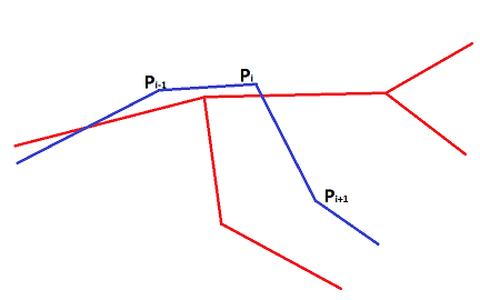
A track is an ordered sequence of points containing some error. Because of this error, the point will almost never lie on the edge of the graph to which you want to bind. According to the law of meanness for GPS data, the positioning error is less in the open field than in the city center. In other words, the arriving point may fall on the adjacent edge.



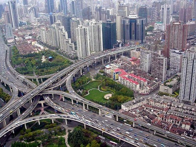
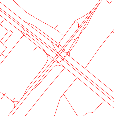
It looks like one Moscow interchange eyes card:





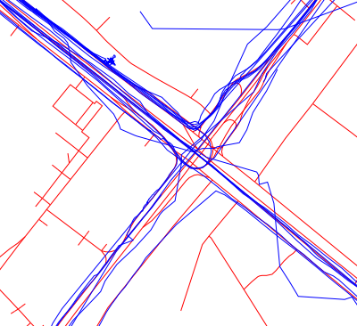
And this is how it is, according to the version of navigators, our users are traveling:

Track binding process

To bind a track point to a graph, in the simplest case, it is necessary to find the edges with the minimum distance from the edge to the point. Unfortunately, in practice (especially in the center of the city), a route bound in this way may turn out to be a set of unlinked edges. In order to improve the quality of the binding, we will assume that the track is the ordered orderly movement of the user along the geometry of the edges of the graph. That is, the entire route passes through the edges connected to each other. In this case, each edge of the route may have several points of the track, or none.



Thus, since we refuse to take the edge closest to the point, we need to choose some other quantitative measure that would allow us to determine how well the measured edge fits.



There are many factors that can be used:

1. The distance from the point to the geometry of the edge of the graph. Estimates both the shortest distance and the probability that the receiver could make such an error.
2. The coincidence of the directions of movement. Estimates the angle between the vehicle's motion vector and the direction of the section of the edge geometry to which the point is attached. (This measure is resistant to the systematic error of the GPS receiver, but is subject to random).
3. Change the direction of the vehicle. The probability that the car will turn off the main road is generally less than the probability that it will continue along it (this is how the number of maneuvers is minimized).
4. The physical ability to go from one edge to another (edge ​​reachability). The adequacy of the speed with which the car had to move to make this transition.

Based on these factors, a likelihood assessment formula is created. Fréchet distance is used as one of such formulas. Simply put, this is the minimum required length of a dog leash, if the owner will go on the road graph, and his pet - on the GPS track. This estimate focuses only on the geographic distance of the track being laid.



To bind tracks in this article, we use the evaluation formula for the incremental data binding algorithm (based on the work of S. Barcatsoulas [2]).



This formula includes two main components: and .



Component It takes into account the weighted distance from the track point to the edge and is calculated by the formula:



where

Are the scaling factors, and Is the distance from point p _i to the geometry of the edge c _j .



Component takes into account the angle between the direction of the geometry of the edge and the direction of the track:



where

and Are the scaling factors, and cos (α _{i, j} ) is the angle between the geometry of the i-th edge of the graph and the direction of movement along the edge of the track

and - These are the parameters that affect the significance of the components. For the algorithm, the values ​​of these parameters relative to each other are important - this determines which of the factors will have more weight when comparing.



Options and affect the sensitivity to changes in the described factor.



After calculating the components, the final metric is calculated as:







The larger the number in the end, the better the coincidence of the track section and the edge.



Having in the arsenal the likelihood formula of the route to be laid, we can describe the binding algorithm:

1. , ;
2. ;
3. . ;
4. , . ( , );
5. ;
6. 2;

Follow-up strategy

The undoubted advantage of the chosen formula is the ability to estimate the likelihood of being tied to a graph not only for one point, but also for the route as a whole. This can be used to implement a strategy for accounting for subsequent points. If at the moment the last point of the route is not linked, then you can calculate the estimates of the binding of the following points, provided that the route runs along the selected edge. After that you can already compare the amount of likelihood estimates. This will avoid errors at difficult intersections and intersections, since the algorithm will choose the edges, taking into account the subsequent movement.

Little about performance

The task of linking a single track is not incredibly costly, but in practice it’s rare that anyone ever ties a pair of tracks. As a rule, it is necessary to have time to link thousands of points per second. Therefore, we have to find a compromise between processing speed and accuracy of track reference. In the selected algorithm, the number of estimated edges for each track point and the depth of evaluation of “from the future” points affect performance. As practice has shown, to make the right decision about behavior at intersections, in most cases it is enough to take into account 2-3 subsequent points of the track.



The number of estimated edges is actually difficult to change, since for a high-quality binding after selecting the first edge, it is necessary to evaluate all outgoing edges. But you can not consider options with too low likelihood.

Results

The implementation of the binding algorithm has enabled the Map@Mail.ru project not only to start working with mobile users' data, but also to quickly coordinate its own data with arbitrary systems. Using the new subsystem of binding allows for a minute on one server to recalculate tracks, totaling up to 55 thousand points, to your graph. Thanks to this, data is displayed to users as quickly as possible. The algorithm shows a qualitative binding even with one point of the track on three edges of the internal graph. However, the highest efficiency of the described algorithm is achieved during the binding of long tracks with one or two points on each edge of the graph.

Related Literature

1. “Map Matching. An Introduction ”Prof. David Bernstein, James Madison university.
2. “On Map-Matching Vehicle Tracking Data” Sotiris Bracatsoulas, Dieter Pfoser Randall Salas Carola Wank VLDB'05
3. “Approximate Map Matching the Frechet Distance” Daniel Chen, Anne Driemel, Leonidas J. Guibas, Andy Nguyen, Carola Wenk. Stanford. 2011

---

Lev Dragunov, programmer