Index method for generating finite discrete distributions
Sometimes it is very interesting to imitate the roll of the dice For this there is an effective algorithm that allows you to generate the value fallen on the upper face, using a pseudo-random number  from even distribution on
 ![[0,1]](https://habrastorage.org/getpro/geektimes/post_images/1e5/668/a24/1e5668a24690f7b412a044dbc14ad6bd.png) . Namely:
. Namely:  where
where  - taking the whole part of the argument.
But suppose that we have a “dishonest” bone and the faces fall out unevenly. Let our bone has K faces, and face loss probability
  . This is a natural limitation.
  . I will try to answer the question: how to simulate a pseudo-random sequence with such a distribution?

')
Consider the "naive" version of the generation of such a distribution. We introduce the concept of partial sums , you can write equality
  . It remains to famous
  and
and  find specific i. If you simply go through all i starting from 1 and ending with K, then on average you need
  comparison operations. In the worst case, which, by the way, meets with probability
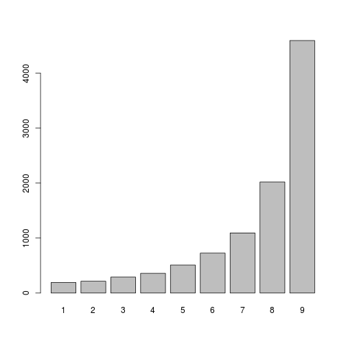
  , we will need K comparisons, for an example from the graph above, it appears with a probability of 0.45473749. On the average, 7.5 comparisons and generation of one random variable are required. The number of operations makes you sad especially if you want to simulate a large number of throws with the wrong bone.
One of the ideas how to solve a bad luck is to pick up such a correct bone, by looking at which we can roughly bring our wrong bone closer and do it very quickly. This method is called the Chen method, and can also be found under the name “cutpoint method” or the “index search” method.
The essence of the method is very simple, divide the segment![[0,1]](http://mathurl.com/a5nwa6n.png) on M equal parts. We introduce an additional array r of length M. In the element
on M equal parts. We introduce an additional array r of length M. In the element  the array will be stored i, such that
  :
:
In this case, the algorithm for generating a new value takes the following form:
In the worst case, for the example above, we will need (with M equal to 9) 4 comparisons with a probability of 0.03712143. On average, one will need to generate one random variable and 1.2 comparisons. If there is a lot of memory and the data preparation stage (task ) is relatively rare, M can be chosen arbitrarily large.
The method is simple to implement and gives a significant gain in the rate of generation of a large number of realizations of the same random variable, especially in the case of a large number of almost identical states. Just in case, a rough implementation on c ++ is laid out on pastebin .
 from even distribution on
 ![[0,1]](https://habrastorage.org/getpro/geektimes/post_images/1e5/668/a24/1e5668a24690f7b412a044dbc14ad6bd.png) . Namely:
. Namely:  where
where  - taking the whole part of the argument.
But suppose that we have a “dishonest” bone and the faces fall out unevenly. Let our bone has K faces, and
 face loss probability
  . This is a natural limitation.
  . I will try to answer the question: how to simulate a pseudo-random sequence with such a distribution?
#Naive approach len<-10 ps<-seq(len,2, by=-1) ps<- 1/ps^2 ps<-ps/sum(ps) ss<-cumsum(ps) gen_naiv <- function() { alpha<-runif(1) return (min(which(alpha<ss))) } #sample val<-c() len<-10000 for(i in 1:len) { val<-append(val, gen_naiv()) } vals<-factor(val) plot(vals) 
')
Consider the "naive" version of the generation of such a distribution. We introduce the concept of partial sums
 , you can write equality
  . It remains to famous
  and
and  find specific i. If you simply go through all i starting from 1 and ending with K, then on average you need
  comparison operations. In the worst case, which, by the way, meets with probability
  , we will need K comparisons, for an example from the graph above, it appears with a probability of 0.45473749. On the average, 7.5 comparisons and generation of one random variable are required. The number of operations makes you sad especially if you want to simulate a large number of throws with the wrong bone.
One of the ideas how to solve a bad luck is to pick up such a correct bone, by looking at which we can roughly bring our wrong bone closer and do it very quickly. This method is called the Chen method, and can also be found under the name “cutpoint method” or the “index search” method.
The essence of the method is very simple, divide the segment
![[0,1]](http://mathurl.com/a5nwa6n.png) on M equal parts. We introduce an additional array r of length M. In the element
on M equal parts. We introduce an additional array r of length M. In the element  the array will be stored i, such that
  :
: #Preprocessing ss<-cumsum(ps) ss<-append(ss, 0, after=0) M<-length(ss) rs<-c() for(k in 0:(M-1)) rs<-append(rs, min(which(ss>=k/M))) In this case, the algorithm for generating a new value takes the following form:
#chen's method finite discrete distribution generator gen_dfd <- function() { M<-10 alpha<-runif(1) idx<-rs[floor(alpha*M)+1] return (idx-1+min(which(alpha<ss[idx:(M+1)]))-1) } #sample code val<-c() len<-10000 for(i in 1:len) { val<-append(val, gen_dfd()) } vals<-factor(val) plot(vals) In the worst case, for the example above, we will need (with M equal to 9) 4 comparisons with a probability of 0.03712143. On average, one will need to generate one random variable and 1.2 comparisons. If there is a lot of memory and the data preparation stage (task
 ) is relatively rare, M can be chosen arbitrarily large.
The method is simple to implement and gives a significant gain in the rate of generation of a large number of realizations of the same random variable, especially in the case of a large number of almost identical states. Just in case, a rough implementation on c ++ is laid out on pastebin .
Source: https://habr.com/ru/post/157689/
All Articles