Interpolation + (linear | logarithmic) scale + С ++

It took me somehow to make an interface for loading into the microcontroller a graph of the function “resistance -> temperature” (they decided to set the graph by several points, and then interpolate them). Along the way, it turned out that the schedule would be very non-linear (180 ohms -> 100 ^o , 6 000 ohms -> 0 ^o , 30 000 ohms -> -30 ^o ). So I had to immerse myself in the subject of logarithmic scales ... and immediately emerge, since I did not find what I needed. And all I needed was to understand mathematics (and the implementation in C ++) of such cases. Wonderful - like this is a necessary topic, but not painted! Well, okay - the brains squeaked and remembered the highest mathematics from the university, and the program was written. I decided to describe my ordeal here - maybe someone will come in handy.

In this article I will write out the theory (as well as the basic virtual classes), next I will take up concrete implementations using Qt tools.

Caution: there are a lot of graphics in the text!

')

Where the legs grow from the task

In general, I need to make an idling regulator - such a thing for a car that, when idling, depending on the temperature of the engine, must maintain certain revolutions. It supports them by adjusting the damper with a stepper motor.

In general, I need to know the current temperature. It was decided to measure it by standard means - with a thermistor. We measure the voltage drop on it - we get resistance. Further from the table (since it is a microcontroller) we get the required speed.

This table must be set (for this program is written by means of Qt). I have a few “resistance => temperature” points. I need for each ADC code (for a number of values of proportions) to obtain the appropriate temperature. Since different cars may have different values, it’s necessary to specify several points on the curve on the screen, referring to the table.

Along the way, it turned out that this graph will be clearly on a logarithmic scale. So you need to display it on the screen. How to do it - read on.

Formulation of the problem

Let's describe in more detail what we need:

setting the function - it is necessary to set several points on which the graph is built. In general, we recall the interpolation ;
plotting a function - yes, yes, I know about Qwt . Maybe not very well, I know him, because I have not found the following opportunity in him:
Interactive task of the function - I need to move the points on which the function is built, directly on the screen, in the current screen coordinates of the scale, which are translated into real value;
linear / logarithmic scale - since the values are what I wrote, I had to lay the possibility of changing the scale. And both one and both at once.

Here is the TK ... Well, nothing, I managed! Let me help you too.

Yes, until dived - thanks to CodeCogs Equation Editor ! With their help, I famously built all the mathematical formulas without any Microsoft Equation Editor, which then still need to be exported to graphics with an insert here. By the way, there is a Russian editor . In general, I recommend!

Well, if instead of formulas you see empty squares, this is also a “thank you” Equation Editor ...

Attached Excel file

In the course of writing this article, I built all the calculations and checked it in the Excel spreadsheet with formulas. It turned out very convenient. And I decided to post it for public use. There are listed at the bottom of the page sections. On each page, the parameters that can be changed are marked as cells with a yellow background. It is better not to touch the remaining cells. However, all formulas can be easily viewed. Download the file and try on health! If problems with the file - write, send.

Functional dependence

So, we have some dependency - we denote it as

. Here we have

- horizontal axis of the graph,

- vertical. In my case

was the value of resistance

- temperature.

Why not

? After all, it seems to be so? That's the way it is, but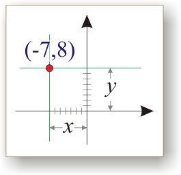 ~~only at school~~ in the simplest case.

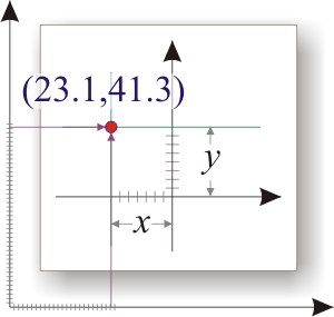- This is the coordinates of a point on the plane. For simplicity, we define the use of the Cartesian coordinate system : $y$ sets the vertical offset of the horizontal axis relative to zero, $x$ sets the horizontal offset of the vertical axis relative to zero.

Everything is good when we draw this very coordinate system on paper and put dots in it. There really - they chose the center, put the ruler here, then there. But when plotting a chart in some program, subtleties begin - what should be considered zero? What is considered a "+", and what is a "-"? I draw graphics for this article in CorelDRAW - there the center is considered from the bottom left (you can move it where necessary).

Yes, and in what units of the schedule? In centimeters? And why? I will have the next stage of implementation in C ++ using Qt tools, so there I will make a QWidget window, which, by default, has a zero - is the top left; units of measurement - screen pixels.

Well, do not forget that all these beautiful arguments are valid for the linear scale so far, and here we have logarithmic looming over the horizon. There the devil knows what will happen!

But this is only a point. And we will have some kind of line, more precisely - many lines. What will be there for the transformation?

That is precisely why we must, from the very beginning, clearly separate the functional dependence and coordinate transformations .

So, let's agree on the following: we have some abstract process, which is described by functional dependence . When displayed on the screen is used to convert to coordinates $(t,f(t))\Rightarrow(X,Y)$ where $X=X(t)$ , $Y=Y(f(t))$ . The next steps are to clarify these

and

.

But let's put the coordinates aside for the time being - do we need to somehow define our function (remember the TK)? And set in those very abstract coordinates

. And this will do.

Interpolation

In my case, a number of points were known.

Ω	˚
180	100
6,000	0
30,000	-thirty

Not so hot, and a large table, but there’s obviously a lot of empty places. And what resistance corresponds to 60˚, -40˚, ...? In general, you need to put the missing points. And interpolation , approximation and extrapolation will help us in this. However, do not worry - one interpolation is enough for the eyes.

There are many interpolation methods, I will not consider everything here. Personally, I liked at the beginning the Lagrange interpolation polynomial . It is very simple in the calculation and implementation, as well as in customization. There it is assumed that a set of

view points

(here we will for a while return to the assignment of points in the form

- so it is accepted in mathematics).

The polynomial is calculated as

where

.

Math scared? Hmm ... Ok, I'll write in C ++:

typedef qreal Real; Real Lagranj (Real X) { static const int n = 3; static Real y[n] = {100, 0, -30}; static Real x[n] = {180, 6000, 30000}; Real L, l; int i, j; L = 0; for (i = 0; i < n; ++i) { l = 1; for (j = 0; j < n; ++j) if (i != j) l *= (X - x[j]) / (x[i] - x[j]); L += y[i] * l; } return L; } int main (int argc, char *argv[]) { Real y; y = Lagranj (180); y = Lagranj (500); y = Lagranj (1000); y = Lagranj (6000); y = Lagranj (10000); y = Lagranj (30000); y = Lagranj (0); y = Lagranj (100000); }

As you can see, everything is rather trivial (how trivial polynomials can be).

Another big advantage of Lagrange polynomials is that they can be easily modeled in an Excel spreadsheet, which I did.

Then, however, everything became a bit sad, since these polynomials, like any others, have vibrations on the graph. That is, they can not give straight lines - constant values. In my case, I could not set them up properly - they were bent into clearly unacceptable numbers. So I had to give them up ...

Working in Corel, I was intimately familiar with Bezier curves — also a fairly convenient and simple representation of tabular data. Very easy to implement in programming. However, this is no longer an interpolation, but rather an approximation, since here one has to adjust the curve to the desired form.

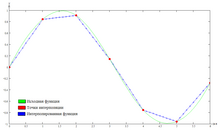As a result, after carefully looking at my function, I realized that I would rather have a piecewise linear interpolation — straight segments between the given lines. Not that it’s really feng shui, but it’s easily realizable and conveniently customizable.

In the language of mathematics, we are between the points

and

draw straight lines of sight $y=y_{i}+\frac{y_{i+1}-y_{i}}{x_{i+1}-x_{i}}(x-x_{i})=k_{i}*x+b_{i}$ .

Again, in C ++ it will look like this:

 typedef qreal Real; Real Linear (Real X) { static const int n = 3; static Real y[n] = {100, 0, -30}; static Real x[n] = {180, 6000, 30000}; static Real k[n] = { (y[1] - y[0]) / (x[1] - x[0]), (y[2] - y[1]) / (x[2] - x[1]), (y[3] - y[2]) / (x[3] - x[2])}; static Real b[n] = { y[0] - k[0] * x[0], y[1] - k[1] * x[1], y[2] - k[2] * x[2]}; int i; // .   ? if (X <= x[0]) return y[0]; else if (X >= x[n-1]) return y[n-1]; // .  ? for (i = 0; i < n-1; ++i) if (X == x[i]) return y[i]; // .  ? for (i = 0; i < n-1; ++i) if (X >= x[i] && X <= x[i + 1]) return k[i] * X + b[i]; return 0; //  -      !!! } int main (int argc, char *argv[]) { Real y; y = Linear (180); y = Linear (500); y = Linear (1000); y = Linear (6000); y = Linear (10000); y = Linear (30000); y = Linear (0); y = Linear (100000); }

Also nothing revolutionary, is it?

There is one significant difference between the Lagrange polynomial and linear interpolation: for the first one, you cannot explicitly specify values outside the points - they are calculated, for the second one you can control this matter. That's why I ended up settling on the linear version. Moreover, on the logarithmic scale I was aiming for, linear segments give me a more suitable option.

However, we will not bother now on interpolation methods. Let's better make a base class from which we will inherit implementations of various ~~$ # * @!~~ polatsii.

Base class for setting / calculating a function

What should this class be able to do? It seems to me that such a class should:

give the value of the function depending on the argument - in fact, for the sake of which we and his city;
react (move and recalculate) to change interpolation points - the fact of pressing / releasing in a certain coordinate is input to the input, as a result of which parameters are recalculated;
to distinguish between single and double mouse clicks - a single press, as for me, indicates the movement of a point; double creates a new point;
to draw interpolation points both during their movement and without it, since different interpolation methods will have different intuitive meaning of interpolation points, then the derived class should derive them (for example, in interpolation the point is part of the graph; in approximation, the point is not necessarily lies on the graph; in the Bezier curves, part of the points lies on the graph, some set the shape);
give the coordinates of the current moving point - this is necessary to display the text coordinates of this point;
give service information - for example, “is a function defined?”, “how many points are used for interpolation?”, “get coordinates of points”, etc. This data will allow you to save current settings;
to make settings - “distribute so many points”, “set coordinates of a point” - this will allow us to restore saved settings.

Any more thoughts? If will be - write in comments, we will add!

It turns out such a class:

 class FunctorBase { protected: virtual QPointF &get_point (const int Pos) = 0; //    virtual QPointF get_point (const int Pos) const = 0; //    public: // .  virtual void MouseClicked (const QPointF &Pt) = 0; //       Pt virtual void MouseDblClicked (const QPointF &Pt) = 0; //        Pt virtual void MouseReleased (void) = 0; //    virtual void MouseMove (const QPointF &Pt) = 0; //   (   ),   Pt virtual void DrawPoints (QPainter &p, const ScaleBase &X, const ScaleBase &Y, const int ptRadius, QPen &pnCircle, QBrush &brCircle) = 0; //    ,   virtual void DrawCurPoint (QPainter &p, const ScaleBase &X, const ScaleBase &Y, const int ptRadius, QPen &pnCircle, QBrush &brCircle) = 0; //     (   ,  ) // .  virtual qreal f (const qreal t) const = 0; //     virtual QPointF *point (void) const = 0; //   ;    -  NULL virtual bool is_specified (void) const = 0; //   virtual int num_points (void) const = 0; //     QPointF point (const int Num) const; //      // .  virtual bool set_points (const int Num) = 0; //   ;    QPointF &point (const int Num); //      void set_point (const int Num, const QPointF &Pt); //       // .   qreal operator() (const qreal t) const { return f(t); } //     operator bool (void) const { return is_specified (); } //   QPointF &operator[] (const int Num) { return point (Num); } //      QPointF operator[] (const int Num) const { return point (Num); } //      }; // class FunctorBase inline QPointF &FunctorBase::point (const int Num) { Q_ASSERT_X (Num < num_points (), "receiving points", (QString ("incorrect point index %1 for array size %2 is used"). arg (Num). arg (num_points())).toAscii().constData()); return get_point (Num); } inline QPointF FunctorBase::point (const int Num) const { Q_ASSERT_X (Num < num_points (), "receiving points", (QString ("incorrect point index %1 for array size %2 is used"). arg (Num). arg (num_points())).toAscii().constData()); return get_point (Num); } void FunctorBase::set_point (const int Num, const QPointF &Pt) { point (Num) = Pt; }

(Those who are dissatisfied with my style and structure - offer objectively better!)
(For those who find errors in the code - thanks!)

I think everything is obvious here.

For coordinates, the point representation in the form of QPointF is used (a pair of numbers in the form of qreal, qreal. "On all platforms except ARM, a double is used" - this is written for Qt 4.8 ).

Mouse button presses are implemented by the MouseClicked , MouseDblClicked , MouseReleased and MouseMove functions. It is assumed that in specific implementations will be the appropriate reactions.

Draw points by using DrawPoints and DrawCurPoint . If the coordinates are used for all methods except these, the abstract ones are used, then we need the most screen ones. Therefore, two ScaleBase for transformation are passed here. This class is also virtual. His ancestors implement the transformation from abstract coordinates to the current screen. This class itself will be described below.

The current value of the function is returned by the f (const qreal) method and the overloaded operator function operator() (const qreal) .

To set the structure, the set_points (Num) functions are used - setting the number of points, point (Num) , set_point (Num) , get_point (Num) - setting the coordinates of a specific point. num_points () const - returns the number of points, point (Num) const , get_point (Num) const returns the coordinates of the point. is_specified () const returns true if the structure of the function is specified.

In the next article we will write a couple of options for implementing this class.

Transform function for vertical / horizontal scale

There are linear and logarithmic scales. Given that the vertical scale can be made in one format, and the horizontal scale in another, we get four options for the graph:

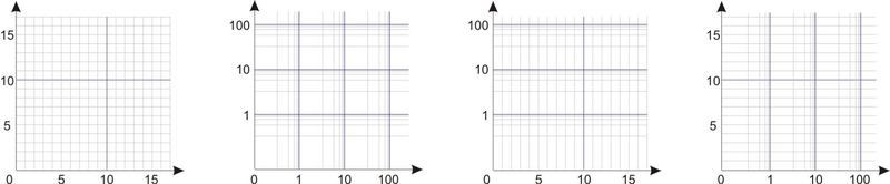
Option one - both scales are linear. Option two - both logarithmic. Options for the third and fourth - mixed graphics. By the way, in my case, it was a mixed case that eventually came up, since horizontally I needed a logarithmic scale, vertically - linear.

Consequently, the mapping problem must be solved separately for both axes.

Recall that when displaying on the screen is used to convert to coordinates $(t,f(t))\Rightarrow(X,Y)$ where $X=X(t)$ , $Y=Y(f(t))$ . Our further task is to construct these functions for the linear and logarithmic cases.

What are these features? At the entrance they get the coordinate in abstract (for the computer subroutine mapping on the screen) coordinates, the output is given in the screen (the "screen" coordinates will be different for different operating systems "). To calculate, they need to know the following:

the limits of abstract coordinates are the limiting values of the argument and function that we are interested in. It will be , for the horizontal axis and , for vertical. No need to make a classic mistake: , ! In the example above, this is illustrated;
The screen coordinates are the borders of the picture in which the graph is drawn. Naturally, in the current screen coordinates. On the chart this $x_{min}$ , $x_{max}$ for the horizontal axis and $y_{min}$ , $y_{max}$ for vertical;
screen coordinate pitch - current pixel pitch $x_{step}$ , $y_{step}$ . In the simplest case, it will be one. But in Qt, vertical zero is the top of the window. Consequently, $y_{step}=-1$ . And any other transformations can be applied, and the step will be far from single.

Please note - for the conversion task it does not matter whether the axis is vertical or not! It (the task) operates on the boundary values of the input, output, and output parameter steps. Therefore, the task can be generalized: it is necessary to convert the parameter based on its limits , output value given its limits , and step . There are intentionally introduced notation.

instead of the usual $x$ , $y$ , because otherwise there will be confusion. One significant addition:

Base class for scale conversions

Let's formulate the desired functionality of the virtual class of transformations for the scale, from which the implementation of the scales will be inherited:

transformations from screen coordinates to abstract and vice versa - it is logical, for the sake of it we do it;
conversion setting is also logical;
properties - current properties of the transformation (minimum / maximum values, step for different values);
information on the grid - positions for large and small grid, the caption under the scale.

The implementation might look like this:

 class ScaleBase { public: // .  virtual qreal scr (const qreal Val) const = 0; //       virtual qreal val (const qreal Scr) const = 0; //       // .  virtual const QVector<qreal> &scr_values (void) const = 0; //   ,  [  (    )] int num_scr_values (void) const; virtual const QVector<int> &scr_min_grid (void) const = 0; //      int num_scr_min_grid (void) const; virtual const QVector<int> &scr_maj_grid (void) const = 0; //      int num_scr_maj_grid (void) const; virtual const QVector<int> &scr_text_pos (void) const = 0; //       int num_scr_text_pos (void) const; virtual const QVector<QString> &scr_text_str (void) const = 0; //       int num_scr_text_str (void) const; // .  virtual qreal val_min (void) const = 0; //     ,    virtual qreal val_max (void) const = 0; //     ,    virtual qreal scr_min (void) const = 0; //      virtual qreal scr_max (void) const = 0; //      virtual bool is_specified (void) const = 0; //   // .  virtual void set_val_min (const qreal Val) = 0; //     ,    virtual void set_val_max (const qreal Val) = 0; //     ,    virtual void set_scr_min (const qreal Src) = 0; //      virtual void set_scr_max (const qreal Src) = 0; //      virtual void set_scr_point (const qreal Src) = 0; //     () // .  void Resized (const qreal Size) = 0; //    // .   operator bool (void) const { return is_specified (); } //   }; // class ScaleBase int ScaleBase::num_scr_values (void) const { return scr_values().size(); } int ScaleBase::num_scr_min_grid (void) const { return scr_min_grid().size(); } int ScaleBase::num_scr_max_grid (void) const { return scr_max_grid().size(); } int ScaleBase::num_scr_text_str (void) const { return scr_text_str().size(); } int ScaleBase::num_scr_text_pos (void) const { return scr_text_pos().size(); } virtual qreal ScaleBase::scr_step (const int Num) const { Q_ASSERT_X (Num < num_scr_values (), "receiving step", (QString ("incorrect step index %1 for array size %2 is used"). arg (Num). arg (num_scr_values())).toAscii().constData()); return scr_values()[Num + 1] - scr_values()[Num]; }

Scale adjustment is performed with the set_... (Val) functions. Recalculation of the necessary values should be made in the same functions. When the window is Resized (Size) method is Resized (Size) .

To improve performance, you can once calculate the compliance point on the screen and its value in the original, abstract coordinates. This array is returned by the scr_values () const method. Further, to build a large and small grid, arrays are calculated (return them, respectively, to the functions scr_maj_grid () and scr_min_grid () ). The length of the array corresponds to the number of these lines, the value - the offset relative to the beginning of the scale on the screen (i.e. the index of the first array). Also, two arrays are pre-calculated - the text of the caption to the scale (the scr_text_str () function) and the offset of these signatures relative to the beginning (the scr_text_pos () function).

Finally, the direct conversion — from abstract to screen coordinates — is performed by the scr (Val) function, and the reverse, by the val function (Scr) .

Linear transform

Let us consider separately the linear transformation for the horizontal and vertical axis.

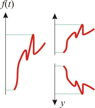
We have a certain function - a curve in one representation. For another, we had to narrow it down and shift it to the right (the window on the screen was reduced and shifted to the right). For another view, we had to shift it to the left (the window was shifted to the left). How is it described mathematically? Simple enough: $y=f(k*t+b)$ . In the first case, it seems

in the second $b<0$ .

In another case, we had to narrow the vertical representation of the curve and move it upwards. And then in general - to turn. Both of these transformations are described as $y=k*f(t)+b$ . In the first case

, $b>0$ . In the second case $k=-1$ .

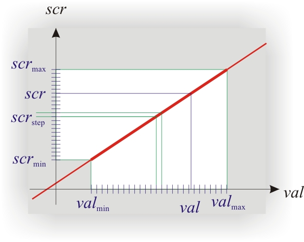
Both transformations have the same mathematical description:

. In this description there are two constants that define the transformation - $k$ and $b$ . The first determines the angle of inclination, the second - the offset relative to zero.

The calculation of these constants is quite simple - this is a solution to a system of two equations:

$\left\{\begin{matrix}scr_{min}=k*val_{min}+b; \\scr_{max}=k*val_{max}+b; \end{matrix}\right. \Rightarrow \left\{\begin{matrix}k=\frac{scr_{min}-scr_{max}}{val_{min}-val_{max}}; \\b=scr_{max}-k*val_{max}; \end{matrix}\right.$

.

It is also important to be able to do the inverse transformation — for example, translate the coordinates of the mouse pointer into abstract coordinates. Also, nothing complicated:

$val=\frac{scr-b}{k}$

.

Step

in this case it is not used for the calculation, but then it will be useful to us in the implementation in C ++ for the calculation of the displacement.

How will this be used in practice? Yes, everything is simple! Horizontal transformation:

- border image graphics corresponding

(usually left)

(usually to the right)

- horizontal image output step. Vertical transformation is the same, but vertically (in Qt

will be the lower border of the picture

- top, and

Logarithmic transformation

And now we will plunge there for the sake of what all this has started to turn:

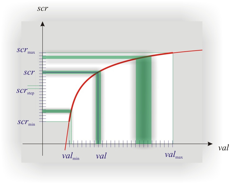
(the graph does not draw a logarithm, but something similar to it. It was done on purpose, since the logarithm will not be very obvious here)

If a

same on the whole scale then

will be different everywhere! What law does it change? That's right - logarithmic! Let's first learn to identify this very

.

Total points we will have $num=\left | \frac{scr_{max}-scr_{min}}{scr_{step}} \right |+1$ (eg,

; then we will have 3 points). This corresponds to the input range. $diap_{val}=val_{max}-val_{min}$ . Value $scr_{0}=scr_{min}$ corresponds to $val_{0}=val_{min}$ , $scr_{n}=scr_{max}$ corresponds to $val_{n}=val_{max}$ . The last point has an index $n=num-1$ . What corresponds to $scr_{i}$ ?

For linear scale $scr_{i}\equiv val_{min}+base*i$ where

determined by the range of input values. Here you can do the same, but instead of multiplication there will be a raising to a power: $scr_i\equiv val_{min}+base^i$ (remember that $0\leqslant i\leqslant n$ ). There is one, however, nuance:

we have

, and should. This is solved simply - subtract one: $scr_i\equiv val_{min}+base^i-1$ . And then for the zero case, everything converges. How to calculate

in this case? There are different options. I prefer to do this as follows.

We know that $scr_n\equiv val_{max}$ . At the same time, we now know that $scr_n\equiv val_{min}+base^n-1$ . It turns out the equation: $val_{max}=val_{min}+base^n-1$ . Solve it for

. Remembering what is

and replacing the root with exponentiation, we obtain an acceptable form for a computer:

(recall that

). Fine, the base value is received!

In fact, we obtained an algorithm for converting from screen to abstract coordinates — the inverse problem. Now the mode of the direct task is the transformation from an abstract coordinate to a screen one. The problem is solved easily. In fact, you need to find

and it's easy for him $scr_i$ .

To find

need to solve the equation

regarding

. Well, then from the properties of the logarithm we get that

. Well and further, considering the screen coordinates as a line with a slope, we get that $scr_i=\frac{scr_{max}-scr_{min}}{n}*i+scr_{min}$ (for more beauty you need more

replaced by

).

It seems to be considered basic math. Found errors or inaccuracies - write in the comments, I will be grateful!

Over time, I will write the following article - the implementation of this mathematics using Qt in C ++.

Source: https://habr.com/ru/post/157407/

All Articles