Filtering false matches between images using a dynamic match graph
Many modern computer vision algorithms are built on the basis of detecting and comparing the special points of visual images. On this topic, many articles were written on Habré (for example, SURF , SIFT ). But in the majority of works, due attention is not paid to such an important stage as filtering of false correspondences between images. Most often for these purposes apply RANSAC-method and stop at this. But this is not the only approach to solve this problem.
This article focuses on one of the alternative ways to filter false matches.
Formulation of the problem
Suppose we have two sets of singular points obtained from two images P and Q with n p and n q points, respectively. Each singular point is a pair p = {p d , p c }. p d - is a local feature of a point (for example, a SURF descriptor), and p c = {x, y} are the coordinates of a singular point.
We have a set of correspondences M = {c i = (i, i ') | c i ∈ C, i ∈ P, i '∈ Q}, constructed with the help of a certain metric (for example, as points with descriptors closest in the Euclidean metric). For each correspondence, we construct a nonnegative evaluation function S c i = f 1 (i d , i ' d ).
For two matches c i = (i, i ') and c j = (j, j'), suppose that the distance between points i and j in the first image and points i 'and j' in the second image l ij and l i ' j ' respectively. Obviously, if these two matches are true, then we can align the image Q with respect to P with the scale factor l ij frasl; l i'j ' , and we say that this pair of matches votes for the scale l ij frasl; l i'j ' . Now suppose that there is a visual image with n correct correspondences corresponding to it, then for each pair of these correspondences the scale factor should be approximately the same. Such a scale will be called the scale coefficient of geometric consistency and denoted by s. The scale factor of the geometric consistency of a pair of matches c i = (i, i ') and c j = (j, j') is expressed as:
S c i c j (s) = f 2 (| l ij - s * l i'j ' |), where f 2 (x) is a non-negative monotonically decreasing function.
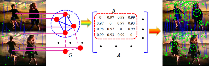
Let the set M contain m correspondences M = {c 1 , ..., c m }. Construct a graph G with m vertices, each vertex of which represents a correspondence from M. The edge weight between vertices i and j is defined as follows:
w ij (s) = S c i * S c j * S c i c j (s).
A graph constructed in this way will be called a Dynamic Conformity Graph (hereinafter referred to as GHS).
')
The weighted adjacency matrix for DGS is denoted by A (s) and constructed as follows:

A (s) ∈ R m * m is symmetric and non-negative.
The correct visual image containing n singular points corresponds to a complete subgraph T ∈ G with n vertices, which, as is easily seen, is a weighted duplicate of the maximum clique. Such a subgraph has a high average intracluster estimate:

If we represent T in the form of an indicator-vector y such that
 , then the average intra cluster estimate can be rewritten in quadratic form:
 where
where  ,
,  .
.As is known, the Motzkin-Strauss theorem establishes a connection between the maximum clique and the local maximum of such a quadratic form:
 where
where  - standard simplex in R m . Simply put, the theorem says that a subset T of vertices of a graph G is a maximal clique if and only if its characteristic vector x T is a local maximum of the quadratic function f (x) in the standard simplex, where x i T = 1⁄ | T | if i ∈ T, x i T = 0 otherwise.
Although the original Motzkin-Strauss theorem applies only to non-weighted graphs, Pavan and Pelillo generalized it to weighted graphs and established a connection between dense subgraphs and local maxima of the equations.
The accepted norm l 1 has a number of advantages. First, it has a simple probabilistic meaning: x i represents the probability that a complete subgraph contains a vertex i. Secondly, the solution x is sparse, and only some components in the same subgraph are of great importance, the other components have sufficiently small values, which allows us to select a cluster by discarding those vertices that are noise, which is noise.
Thus, the task of filtering correspondences is reduced to the problem of finding clusters of correspondences representing separate visual images. In turn, to find such clusters, it is necessary to solve the optimization problem described above.
Algorithm Description
For scale s 0 , the optimization problem
 may have many local maxima. Each large local maximum most often corresponds to the correct visual image, and a small local maximum most often occurs as a result of noise.
When initializing x (1), the corresponding local solution x can be effectively obtained using the first-order self-assembly equation, which has the form:
It can be noted that the simplex Δ is invariant with respect to such dynamics, which means that any trajectory starting from Δ will remain in Δ. In addition, it was proved that when A (s 0 ) is symmetric and with nonnegative elements, the objective function
strictly increases along any non-constant trajectory of the self-assembly equation, and these asymptotically stable points are in strict one-to-one correspondence with local solutions of a quadratic function.Roughly speaking, in order to find all the large local maxima of x, many initial initializations are taken and thus ensure that all the large local maxima of a given simplex will be taken into account. As mentioned above, for our task, each local maximum corresponds to a visual image, then it must have two properties:
- Locality property. The singular points of one visual image lie in a certain small neighborhood, therefore we need to initialize x (1) only in the neighborhood of each vertex of the GVD.
- Non-intersection property. Different visual images, as a rule, do not contain common vertices in G, which means that if two local maxima x and y correspond to two different visual images, then (x, y) ~ 0.
Since we initialized x (1) for each vertex of the DGS and initialization of the vertices of the same visual image converge to approximately the same local maximum, we must merge the local maxima corresponding to the same visual images. Due to this data redundancy, additional noise resistance is achieved. All small local maxima corresponding to noise are also discarded.
At the end, it is necessary to restore the visual image for each local maximum x. Since x i is the probability of occurrence of the vertex i in the visual image x, we can choose only those vertices whose entry into the visual image is most likely.
Algorithm parameters
As can be seen from the above description, the algorithm has a large number of adjustable parameters such as:
- S c i = f 1 (i d , i ' d ) is a function of conformity assessment
- S c i c j (s) = f 2 (| l ij - s * l i'j ' |) is a function for evaluating the geometric consistency of correspondences
- Ε is the threshold value for estimating the weight of the edge, for belonging to the initialization vicinity
- Φ - the radius of the neighborhood for which the initialization x (1) is taken
- Ψ - threshold value for estimating the smallness of the local maximum
- Ω - threshold value for merging neighborhoods
- Θ - threshold value of the probability of occurrence of the vertex in the visual image
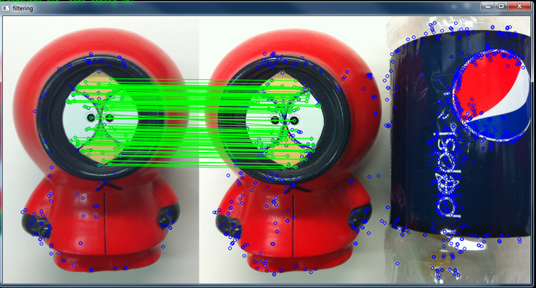
Experiments
Typical results of the algorithm are presented below.
Conclusion
The application of the described algorithm in practice is difficult because of the high sensitivity to the parameters of the algorithm, which are chosen empirically for each set of input data. Also, for the effective application of this method, a preliminary analysis of the input set of correspondences for the selection of the dominant scale factors is necessary.
Due to the fact that the fight against noise occurs due to data redundancy, the algorithm requires a large amount of additional memory and time to process it.
Therefore, this algorithm is interesting from the point of view of the approaches used in it to the analysis of correspondences, and not as an alternative, for example, to the RANSAC method mentioned at the beginning of the article.
Literature
- Spanally Correspondences of Hairong Liu, Shuicheng Yan, National University of Singapore, Singapore
- T. Motzkin and E. Straus. Maxima for the Theorem of Turan. Canad. J. Math, 1965.
- 10. M. Pelillo, K. Siddiqi, and S. Zucker. Matching hierarchical structures using association graphs. TPAMI, 1999.
UPD Link to method sources: dl.dropbox.com/u/15642384/src.7z
Source: https://habr.com/ru/post/154975/
All Articles