How is the short-term forecast for Yandex.Probka
Information about traffic jams appeared on Yandex in 2006. We started with the necessary things - we learned how to build a scheme of congestion of city streets and to take into account the current situation when plotting routes . Driving by looking at this information, motorists could already save time on the road:
Then, to help drivers directly on the road, we added automatic rebuilding of the route to mobile Yandex.Maps (and, as a result, on Yandex.Navigator ). Applications have learned to adapt the route with each noticeable change in the situation in the city.
Having gathered on the desktop and mobile information about the "now", we went to the solution of the question "how will it be then?”:

')
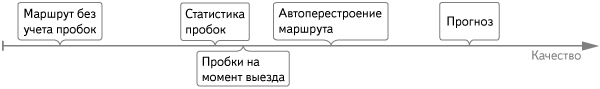
The first step was the statistical map of traffic jams - you can see on it how the city costs and travels on average at a specific hour of a particular day of the week. We assumed that the map of “ordinary” traffic jams could have a useful side effect — the ability to predict traffic jams for them in the near future. But practice has shown that the averaged picture helps to plan approximately, for example, tomorrow's trip to the airport - but it does not help those who are leaving now to avoid new traffic jams. According to our measurements, even at the end of the hourly route, the picture of traffic jams at the time of departure is usually closer to the actual than the average:
A week ago, Yandex.Maps had the opportunity to see the changes in traffic jams in the next hour - our next step in deciding about the future. For those who couldn’t come to the Yet Another Conference this year, we’ll tell you today what our forecast is inside and how it turned out.
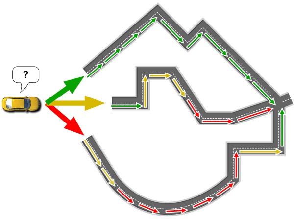
We predict changes in the average speed of movement on different parts of the road. Technically, the road map is a graph. Each intersection - the top of this graph, and the sections of the road between the two intersections - edges. The latter have the attribute "length" and the attribute "speed". The length, of course, is known in advance, and the speed is calculated in real time - depending on it, the section of the road is colored in green, yellow and red. Actually, the second attribute we undertook to predict.
Of course, this task was not invented by us, it is being done by various specialists around the world. In Russia, for example, the authors of a textbook on one of the main directions in this area - “Introduction to Mathematical Modeling of Transport Flows” are working on modeling and forecasting traffic. And although the topic is known for a long time, the car navigation is not available to the Russian user, which uses forecasts based on recent data. Only in rare cases when building a route is taken into account the average statistics of traffic jams.
In the world, workload forecasts are used for automatic traffic control in some cities. The first prototypes in which the forecasts were applied appeared in 1998 in the USA. And the first pilot use of the system, “looking into the future,” began in 2006 in Singapore.
We first touched on forecasting in the Internet Mathematics competition in 2010. That experience helped us understand how the task should be set and what data is needed to achieve a good result.
In many countries, stationary flow sensors are used, which measure the speed and density of traffic on key highways. This is a good source of clean traffic data, but covering even Moscow alone would require huge investments. We completely managed impersonal GPS-tracks that come from users of mobile Maps and Navigator. Each track is a chain of signals about the location (latitude and longitude) of the car at a particular time. We link GPS tracks to a road graph , that is, we determine which streets they passed. Then we average the speed of all the tracks running along the same edges.
This data has a number of features that make it difficult to obtain a qualitative forecast. Consumer GPS-devices determine the coordinates with an error, so the tracks are very "noisy." This complicates not only the calculation of average speeds, but also the binding of tracks to the graph, for example, when the roads pass close to each other:

In addition, sometimes on some streets there are few cars that transmit data. And the situation on the roads itself is not always stable. For example, the lanes of highways move at different speeds, so in the same area tracks can simultaneously show significantly different speeds.
A wide variety of methods are used in this area. Among them:
Parametric regression model . It assumes in advance a specific type of function depending on V future = F ( V past , V current ), and parameters in F are selected. The peculiarity of the model is that the choice of function imposes limitations on the result. On the one hand, it protects against serious errors that are inevitable when using noisy data - the parametric function allows to reduce the spread of the predicted values. On the other hand, with the wrong choice of function, the model can give systematically incorrect answers.
Non-parametric model ( "k nearest neighbors" ). She is simply looking for a situation similar to the current one in the past and, as a forecast, shows how events developed further. Such a model is more flexible - using it, you can say: “If a storm arose 10 times after a lull, then after a new lull there will also be a storm”. If, for example, we take a linear function in a parametric model , we cannot predict this, since it is limited by the hypothesis that the future can only be a linear combination of the past. However, on “noisy” data, the linear model provides greater accuracy than the non-parametric one.
Another classification of regression methods is scalar and vector . In the first, it is assumed that the situation in the selected area does not depend on what is happening on the neighboring, secondly, on the contrary, the dependencies are taken into account. Hence the difference in the amount of calculations. If there are 10 thousand road sections in a city, then to build a scalar model, it suffices to choose 10 thousand parameters. And for a vector model, up to 100 million parameters may be needed. In our case, it is obvious that situations in different areas affect each other. And the key is the question of how to limit the circle of neighbors, so that the calculation went within a reasonable time.
Methods for modeling flows take into account the nature of the process, and not just operate with abstract numbers. The equation of the current fluid with variable viscosity is used: more density - less speed. Methods are widely used for road planning and are promising for forecasts, but are too demanding on accuracy and completeness of data. They give good quality on streaming sensors, but almost do not work on “noisy” GPS tracks.
Experimenting with different methods and evaluating their accuracy and computational complexity, we stopped at linear vector autoregression. It assumes that the future speed is a linear combination of the current and several past speeds in several areas: directly on the considered one, as well as neighboring ones.
Once a day, our model is trained. Based on the development of events for some time period in the past, it builds a forecast. This forecast is compared with subsequent developments. In the model, coefficients are selected in order to minimize the discrepancy between the forecast and how everything actually turned out. For each time of day, the system calculates its coefficients, since the nature of movement during the day varies slightly. Every few minutes, the forecast for the next hour is calculated using the finished model and fresh tracks.
When training the model uses a huge amount of data. The graph of roads takes about 100 gigabytes: this is information about the topology - which edge is connected with which, and also the geometry - the GPS coordinates of the beginning, end, and bend points of each road segment. The history of the tracks, which we store, takes dozens of terabytes. On such volumes, the selection of coefficients for days would stretch out on one server for 2 weeks. To keep within an acceptable few hours, we use a cluster of 30 servers. But in our task it is impossible to simply divide the input data equally between the servers, provide each server with a complete calculation cycle for its part, and collect the final results. Our distributed computing platform helps. It takes on the collection and redistribution of intermediate results, it also automatically transfers tasks from failed servers to working servers and greatly simplifies scaling with an increase in the volume of calculations.
But even with parallelization, such volumes, of course, do not fit in the RAM. Therefore, we use our own Memory Mapped Storage library, which allows an application to work with data on disk as if it were stored in RAM.
Usually we duplicate any data processing between several data centers (DC), so that a failure in any of them does not lead to the inaccessibility of the service for the user. But in preparing the model, we deliberately did not do that. The quality of the forecast will hardly suffer if you use the yesterday model for a few hours. But the forecast itself must always be fresh - the situation on the road is constantly changing. Therefore, it is prepared with triple duplication of calculations in different DCs, completely autonomously from each other. Even if a failure occurs simultaneously in two DCs, the user will not notice. The results of the calculation of different replicas are not synchronized with each other, for each request simply takes the most recent of the three forecasts.
A new forecast is calculated every 10 minutes. First, fresh tracks from users are processed: they are tied to the graph, the speed averaging of cars passing by one segment, the forecast is calculated from the model built for the current day. It takes 1-2 minutes. Then this data is prepared for drawing traffic jams on the map. Sharp drops of speed are smoothed; color is selected for each speed, taking into account the category of roads and the scale of viewing the map. It takes another 2 minutes.
Reliable measurement of forecast quality is in itself an interesting task. After studying several techniques, we chose the following.
The quality metric should reflect how much the forecast helps people. In the absence of a forecast, trying to predict the speed of movement on a road in an hour, we are forced to use current information about traffic jams. It is clear that within an hour the traffic jams will change and our assessment will be incorrect. The estimate obtained using the forecast is also not ideal, but it should be closer to reality. How much closer - we will try to measure it.

Note that you can take different approximations of the actual situation. The simplest is to rely on custom tracks. So we got a rating of 15%.
However, the data itself may have systematic deviations. Then our quality metric will prefer the forecast that diligently reproduces these deviations. To avoid this, we took measurements of assessors - special people who help to measure the quality of service. They traveled on cars with high-precision GPS-devices on the most significant highways, and brought tracks. Comparing the forecast with the assessors tracks, we received a different quality rating - 12%.

Anyone who is seriously interested in the topic of data analysis can recommend the classic textbook The Elements of Statistical Learning (Hastie, T., Tibshirani, R., Friedman, J. - Springer . You can find more detailed information on all the methods of machine learning used in our research.
A large number of materials in Russian is on the site MachineLearning.ru .
A good tutorial edited by A.V. Gasnikova , Introduction to Mathematical Modeling of Transport Flows .
Experts will be interested in the results of foreign research teams involved in the subject of traffic situation forecasting. Of the many publications available, we would like to highlight a few:
Then, to help drivers directly on the road, we added automatic rebuilding of the route to mobile Yandex.Maps (and, as a result, on Yandex.Navigator ). Applications have learned to adapt the route with each noticeable change in the situation in the city.
Having gathered on the desktop and mobile information about the "now", we went to the solution of the question "how will it be then?”:
')
The first step was the statistical map of traffic jams - you can see on it how the city costs and travels on average at a specific hour of a particular day of the week. We assumed that the map of “ordinary” traffic jams could have a useful side effect — the ability to predict traffic jams for them in the near future. But practice has shown that the averaged picture helps to plan approximately, for example, tomorrow's trip to the airport - but it does not help those who are leaving now to avoid new traffic jams. According to our measurements, even at the end of the hourly route, the picture of traffic jams at the time of departure is usually closer to the actual than the average:
A week ago, Yandex.Maps had the opportunity to see the changes in traffic jams in the next hour - our next step in deciding about the future. For those who couldn’t come to the Yet Another Conference this year, we’ll tell you today what our forecast is inside and how it turned out.
Actually, the task
We predict changes in the average speed of movement on different parts of the road. Technically, the road map is a graph. Each intersection - the top of this graph, and the sections of the road between the two intersections - edges. The latter have the attribute "length" and the attribute "speed". The length, of course, is known in advance, and the speed is calculated in real time - depending on it, the section of the road is colored in green, yellow and red. Actually, the second attribute we undertook to predict.
Of course, this task was not invented by us, it is being done by various specialists around the world. In Russia, for example, the authors of a textbook on one of the main directions in this area - “Introduction to Mathematical Modeling of Transport Flows” are working on modeling and forecasting traffic. And although the topic is known for a long time, the car navigation is not available to the Russian user, which uses forecasts based on recent data. Only in rare cases when building a route is taken into account the average statistics of traffic jams.
In the world, workload forecasts are used for automatic traffic control in some cities. The first prototypes in which the forecasts were applied appeared in 1998 in the USA. And the first pilot use of the system, “looking into the future,” began in 2006 in Singapore.
We first touched on forecasting in the Internet Mathematics competition in 2010. That experience helped us understand how the task should be set and what data is needed to achieve a good result.
Data source
In many countries, stationary flow sensors are used, which measure the speed and density of traffic on key highways. This is a good source of clean traffic data, but covering even Moscow alone would require huge investments. We completely managed impersonal GPS-tracks that come from users of mobile Maps and Navigator. Each track is a chain of signals about the location (latitude and longitude) of the car at a particular time. We link GPS tracks to a road graph , that is, we determine which streets they passed. Then we average the speed of all the tracks running along the same edges.
This data has a number of features that make it difficult to obtain a qualitative forecast. Consumer GPS-devices determine the coordinates with an error, so the tracks are very "noisy." This complicates not only the calculation of average speeds, but also the binding of tracks to the graph, for example, when the roads pass close to each other:
In addition, sometimes on some streets there are few cars that transmit data. And the situation on the roads itself is not always stable. For example, the lanes of highways move at different speeds, so in the same area tracks can simultaneously show significantly different speeds.
Method selection
A wide variety of methods are used in this area. Among them:
Parametric regression model . It assumes in advance a specific type of function depending on V future = F ( V past , V current ), and parameters in F are selected. The peculiarity of the model is that the choice of function imposes limitations on the result. On the one hand, it protects against serious errors that are inevitable when using noisy data - the parametric function allows to reduce the spread of the predicted values. On the other hand, with the wrong choice of function, the model can give systematically incorrect answers.
Non-parametric model ( "k nearest neighbors" ). She is simply looking for a situation similar to the current one in the past and, as a forecast, shows how events developed further. Such a model is more flexible - using it, you can say: “If a storm arose 10 times after a lull, then after a new lull there will also be a storm”. If, for example, we take a linear function in a parametric model , we cannot predict this, since it is limited by the hypothesis that the future can only be a linear combination of the past. However, on “noisy” data, the linear model provides greater accuracy than the non-parametric one.
Another classification of regression methods is scalar and vector . In the first, it is assumed that the situation in the selected area does not depend on what is happening on the neighboring, secondly, on the contrary, the dependencies are taken into account. Hence the difference in the amount of calculations. If there are 10 thousand road sections in a city, then to build a scalar model, it suffices to choose 10 thousand parameters. And for a vector model, up to 100 million parameters may be needed. In our case, it is obvious that situations in different areas affect each other. And the key is the question of how to limit the circle of neighbors, so that the calculation went within a reasonable time.
Methods for modeling flows take into account the nature of the process, and not just operate with abstract numbers. The equation of the current fluid with variable viscosity is used: more density - less speed. Methods are widely used for road planning and are promising for forecasts, but are too demanding on accuracy and completeness of data. They give good quality on streaming sensors, but almost do not work on “noisy” GPS tracks.
Experimenting with different methods and evaluating their accuracy and computational complexity, we stopped at linear vector autoregression. It assumes that the future speed is a linear combination of the current and several past speeds in several areas: directly on the considered one, as well as neighboring ones.
What and how is calculated
Once a day, our model is trained. Based on the development of events for some time period in the past, it builds a forecast. This forecast is compared with subsequent developments. In the model, coefficients are selected in order to minimize the discrepancy between the forecast and how everything actually turned out. For each time of day, the system calculates its coefficients, since the nature of movement during the day varies slightly. Every few minutes, the forecast for the next hour is calculated using the finished model and fresh tracks.
When training the model uses a huge amount of data. The graph of roads takes about 100 gigabytes: this is information about the topology - which edge is connected with which, and also the geometry - the GPS coordinates of the beginning, end, and bend points of each road segment. The history of the tracks, which we store, takes dozens of terabytes. On such volumes, the selection of coefficients for days would stretch out on one server for 2 weeks. To keep within an acceptable few hours, we use a cluster of 30 servers. But in our task it is impossible to simply divide the input data equally between the servers, provide each server with a complete calculation cycle for its part, and collect the final results. Our distributed computing platform helps. It takes on the collection and redistribution of intermediate results, it also automatically transfers tasks from failed servers to working servers and greatly simplifies scaling with an increase in the volume of calculations.
But even with parallelization, such volumes, of course, do not fit in the RAM. Therefore, we use our own Memory Mapped Storage library, which allows an application to work with data on disk as if it were stored in RAM.
Usually we duplicate any data processing between several data centers (DC), so that a failure in any of them does not lead to the inaccessibility of the service for the user. But in preparing the model, we deliberately did not do that. The quality of the forecast will hardly suffer if you use the yesterday model for a few hours. But the forecast itself must always be fresh - the situation on the road is constantly changing. Therefore, it is prepared with triple duplication of calculations in different DCs, completely autonomously from each other. Even if a failure occurs simultaneously in two DCs, the user will not notice. The results of the calculation of different replicas are not synchronized with each other, for each request simply takes the most recent of the three forecasts.
A new forecast is calculated every 10 minutes. First, fresh tracks from users are processed: they are tied to the graph, the speed averaging of cars passing by one segment, the forecast is calculated from the model built for the current day. It takes 1-2 minutes. Then this data is prepared for drawing traffic jams on the map. Sharp drops of speed are smoothed; color is selected for each speed, taking into account the category of roads and the scale of viewing the map. It takes another 2 minutes.
Quality control
Reliable measurement of forecast quality is in itself an interesting task. After studying several techniques, we chose the following.
The quality metric should reflect how much the forecast helps people. In the absence of a forecast, trying to predict the speed of movement on a road in an hour, we are forced to use current information about traffic jams. It is clear that within an hour the traffic jams will change and our assessment will be incorrect. The estimate obtained using the forecast is also not ideal, but it should be closer to reality. How much closer - we will try to measure it.
Note that you can take different approximations of the actual situation. The simplest is to rely on custom tracks. So we got a rating of 15%.
However, the data itself may have systematic deviations. Then our quality metric will prefer the forecast that diligently reproduces these deviations. To avoid this, we took measurements of assessors - special people who help to measure the quality of service. They traveled on cars with high-precision GPS-devices on the most significant highways, and brought tracks. Comparing the forecast with the assessors tracks, we received a different quality rating - 12%.
Recommended literature
Anyone who is seriously interested in the topic of data analysis can recommend the classic textbook The Elements of Statistical Learning (Hastie, T., Tibshirani, R., Friedman, J. - Springer . You can find more detailed information on all the methods of machine learning used in our research.
A large number of materials in Russian is on the site MachineLearning.ru .
A good tutorial edited by A.V. Gasnikova , Introduction to Mathematical Modeling of Transport Flows .
Experts will be interested in the results of foreign research teams involved in the subject of traffic situation forecasting. Of the many publications available, we would like to highlight a few:
- Wanli Min, Laura Wynter, Yasuo Amemiya - Road Traffic Prediction with Spatio-Temporal Correlations . This IBM Research Department article describing successful experiences with autoregression helped us believe in the solvability of traffic jams prediction.
- RJ Gibbens, Y. Saacti - Road traffic analysis using MIDAS data route prediction . The report of the research team of the University of Cambridge contains an experimental comparison of the linear regression method and the method of k nearest neighbors.
- Weizhong Zheng, Der-Horng Lee and Qixin Shi - Short-Term Freeway Traffic Flow Prediction: Bayesian Combined Neural Network Approach . In addition to the methods described by us, there are many other approaches to the task of predicting the traffic situation. For example, this article describes the successful experience of using neural networks.
- Yang Zhang, Yuncai Liu - Comparison of Parametric and Nonparametric Techniques for Non-peak Traffic Forecasting . Here a few more parametric and non-parametric forecasting methods are compared.
Source: https://habr.com/ru/post/153631/
All Articles