Through thorns to Haskell. 1/2

The first part is a short and hard introduction to Haskell. The second part can be found here.
tl; dr : A very brief and concise introduction to Haskell.
')
- Introduction
- Haskell Minimum Required
- Tricky part
UPD. If you like the tutorial, drop a few lines to the author of the original article . Man will be pleased;)
I truly believe that every developer should learn Haskell. I do not think everyone should be a super-Haskell Ninja. People just need to know about the opportunities that Haskell opens up. Learning Haskell expands your mind.
The basis of mainstream languages is very similar.
- variables
- cycles
- pointers (even if most languages try to hide this fact, it still remains a fact)
- structures, objects and classes (in most languages)
Haskell is very different. This language uses a bunch of concepts that I have never heard of before. Many of these concepts will help you become a better programmer.
But learning Haskell can be hard. At least it was difficult for me. And in this article I will try to show what I lacked in the process of studying.
This article will be difficult to master. This was done on purpose. There are no easy ways to learn Haskell. This road is difficult and intricate. But I think this is good. Because it is the complexity of Haskell that makes it interesting.
The usual method of learning Haskell is to read two books.
First “Learn You a Haskell” , and then “Real World Haskell” .
I agree that this is the right approach to learning. But in order to understand what Haskell is, you’ll have to read these books very carefully.
On the other hand, this article is a very brief and concise introduction to all major aspects of Haskell. I also added some nuances that I lacked when learning Haskell.
The article consists of five parts:
- Introduction: A short example to show that Haskell may not be scary.
- The very basics of Haskell: Haskell syntax and some basic structures.
- The difficult part:
- Functional style; An example with the transition from imperative to functional style
- Types; types and standard binary tree example
- Infinite structures; Work with an endless binary tree!
- Damn hard part:
- We deal with IO; Minimal example
- Parsing trick with IO; unobvious little thing that kept me from understandingIO
- Monads; unrealistically powerful abstraction tool
- Application:
- A few more words about endless trees; mathematically oriented discussion of infinite trees
Note: Every time you see a delimiter with a file name and a.lhsextension,
You can download it.
If you save the file asfilename.lhs, you can run it with
runhaskell filename.lhs
Some examples may not work, but most should.
Below you should see a link to the file.
01_basic / 10_Introduction / 00_hello_world.lhs
Introduction
Installation

- The Haskell Platform is the standard way to install Haskell.
Utilities:
ghc: A compiler similar to gcc forCghci: Haskell interactive shell (REPL)runhaskell: Run the program without compiling it. Convenient, but very slow compared to compiled programs.
No panic

Many books and articles begin their acquaintance with Haskell with some esoteric formulas (quick sort, Fibonacci, etc.). I will act differently. I will not immediately show Haskell's superpower. I will focus on things in which Haskell is similar to other programming languages. So let's start with the familiar “Hello World”.
main = putStrLn "Hello World!" To run it, save this code as
hello.hs and execute: ~ runhaskell ./hello.hs Hello World! You can download the source at the link that is under the "Introduction"
Save the
00_hello_world.lhs file and execute: ~ runhaskell 00_hello_world.lhs Hello World! 01_basic / 10_Introduction / 00_hello_world.lhs
01_basic / 10_Introduction / 10_hello_you.lhs
And now we’ll write a program that asks for your name and says “Hi, name!”:
main = do print " ?" name <- getLine print (" " ++ name ++ "!") To begin with, let's compare our example with other imperative languages:
# Python print " ?" name = raw_input() print " %s!" % name # Ruby puts " ?" name = gets.chomp puts " #{name}!" // In C #include <stdio.h> int main (int argc, char **argv) { char name[666]; // <- ! // , 665 ? printf(" ?\n"); scanf("%s", name); printf(" %s!\n", name); return 0; } The structure of the programs is very similar, but there are minor syntactic differences. The main part of the tutorial will be devoted to these differences.
In Haskell, each function and object has its own type.
The type of the
main function is IO () .This means that when executed,
main creates side effects.But do not forget that Haskell can look like an ordinary imperative language.
01_basic / 10_Introduction / 10_hello_you.lhs
01_basic / 10_Introduction / 20_very_basic.lhs
Most basic haskell
Before we continue, I would like to warn you about some of the characteristic features of Haskell.
Functionality
Haskell is a functional language.
If you started with imperative languages, you will have to learn a lot of new things.
Fortunately, many of these concepts will help you to program better even in imperative languages.
Advanced static typing
Instead of standing in your way as in
C , C++ or Java , the type system will help you.Purity
Generally speaking, your functions will not change anything in the outside world.
On the one hand, this means that functions cannot change the value of a variable, cannot receive data from the user, cannot write on the screen, cannot launch rockets.
On the other hand, we get easy parallelization of our programs.
Haskell makes a clear distinction between pure functions and functions that produce side effects.
With this approach, it becomes much easier to analyze the properties of your program.
In functionally clean parts of the program, many errors will be eliminated at the compilation stage.
Moreover, functionally pure functions follow the basic Haskell law:
Calling a function with the same parameters will always give the same result.
Laziness
Default laziness is a very unusual thing in programming languages.
By default, Haskell calculates a value only when it is actually needed.
As a result, we have the ability to very easily work with infinite data structures.
The last warning will be about how to read the Haskell code.
For me, this is similar to reading scientific articles.
Some parts may be simple and clear, but if you see the formula, concentrate and read more slowly.
When learning Haskell, it really doesn’t matter if you don’t fully understand some of the syntaxist’s features.
If you meet
>>= , <$> , <- or other scary characters, just ignore them and try to understand the general idea of the code.Definition of functions
You can define functions as follows:
On
C : int f(int x, int y) { return x*x + y*y; } In Javascript:
function f(x,y) { return x*x + y*y; } In Python:
def f(x,y): return x*x + y*y On Ruby:
def f(x,y) x*x + y*y end On Scheme:
(define (fxy) (+ (* xx) (* yy))) And finally, Haskell:
fxy = x*x + y*y Very clear. Neither brackets, nor
def .Remember that Haskell makes extensive use of functions and types.
And therefore it is very easy to define them.
The language syntax was thought out in order to make the definition as simple as possible.
An example of creating a new type
Usually when writing programs, you specify the type of function.
But this is optional.
The compiler is smart enough to do it for you.
Let's play a little.
-- :: f :: Int -> Int -> Int fxy = x*x + y*y main = print (f 2 3) ~ runhaskell 20_very_basic.lhs 13 01_basic / 10_Introduction / 20_very_basic.lhs
01_basic / 10_Introduction / 21_very_basic.lhs
Now try
f :: Int -> Int -> Int fxy = x*x + y*y main = print (f 2.3 4.2) You will get an error:
21_very_basic.lhs:6:23: No instance for (Fractional Int) arising from the literal `4.2' Possible fix: add an instance declaration for (Fractional Int) In the second argument of `f', namely `4.2' In the first argument of `print', namely `(f 2.3 4.2)' In the expression: print (f 2.3 4.2) The problem is that
4.2 is not int.01_basic / 10_Introduction / 21_very_basic.lhs
01_basic / 10_Introduction / 22_very_basic.lhs
One solution would not explicitly indicate the type of the function
f .Then Haskell will print the most common type for us:
fxy = x*x + y*y main = print (f 2.3 4.2) Earned!
Great, we don’t need to create a new function for each data type.
For example, in
C , you would need to create a function for int , for float , for long , for double , etc.But what type should we specify?
To understand which type Haskell brought us, just run ghci:
% ghci GHCi, version 7.0.4: http://www.haskell.org/ghc/ :? for help Loading package ghc-prim ... linking ... done. Loading package integer-gmp ... linking ... done. Loading package base ... linking ... done. Loading package ffi-1.0 ... linking ... done. Prelude> let fxy = x*x + y*y Prelude> :type f f :: Num a => a -> a -> a Hmm ... What is this weird type?
Num a => a -> a -> a At first we will pay attention to the right part
a -> a -> a .To understand it, let's look at a few examples:
| Specified type | Value |
Int | Int type |
Int -> Int | a function that takes an Int as input and returns an Int |
Float -> Int | function that takes an input Float and returns an Int |
a -> Int | the type of the function that accepts any type of input and returns an Int |
a -> a | the type of the function, which takes type a as input and returns the result of type a |
a -> a -> a | the type of the function that takes two arguments of type a as input and returns the result of type a |
In the type
a -> a -> a , the letter a is a type variable .This means that
f is a function of two arguments, and both arguments, as well as the result, have the same type.A variable of type
a can take values of various types.For example
Int , Integer , Float ...So instead of hard typing the type, as in
C and separately define functions for int , long , float , double , etc. ...We simply create one function, as in a dynamically typed language.
Generally speaking,
a can be of any type.String , Int , more complex type, such as Trees , type of another function, etc.But in our example, the type has the prefix
Num a => .Num is a type class .Class type can be represented as a set of types.
Num includes only types that behave like numbers.More strictly,
Num is a class containing types that implement a given set of functions, in particular (+) and (*) .Type classes are a very powerful element of the language.
With their help, we can create amazing things.
But we'll talk about this a little later.
So, the entry
Num a => a -> a -> a means:Let
a be a type belonging to the class of types Num .This is a function that takes input
a and returns ( a -> a ).Well, weird.
In fact, in Haskell no function takes two arguments as input.
Instead, all functions have only one argument.
But note that the function of the two arguments can be represented as a function that takes the first argument and returns a function that takes the second argument as a parameter.
.
That is,
f 3 4 equivalent to (f 3) 4 .Please note that
f 3 is also a function: f :: Num a :: a -> a -> a g :: Num a :: a -> a g = f 3 gy ⇔ 3*3 + y*y You can also use another entry to create a function.
Lambda expressions allow you to create functions without naming them.
They are also called anonymous functions.
We can write:
g = \y -> 3*3 + y*y The
\ character is used because it is similar to the λ character, but at the same time it is an ASCII character.If functional programming is new to you, by this point your brain starts to boil.
It's time to write a real application.
01_basic / 10_Introduction / 22_very_basic.lhs
01_basic / 10_Introduction / 23_very_basic.lhs
But before we start, we need to check that the type system works as it should:
f :: Num a => a -> a -> a fxy = x*x + y*y main = print (f 3 2.4) This code works because
3 can represent either a Fractional (fractional) number of type Float, or an integer of type Integer.Since
2.4 is of type Fractional, 3 also represented as a Fractional number.01_basic / 10_Introduction / 23_very_basic.lhs
01_basic / 10_Introduction / 24_very_basic.lhs
If we register other types in the function, it will stop working:
f :: Num a => a -> a -> a fxy = x*x + y*y x :: Int x = 3 y :: Float y = 2.4 main = print (fxy) -- , x ≠ y The compiler signals an error.
Two parameters must be of the same type.
If you think this is a bad idea, and the compiler should convert the types for you, you really should see a great and funny video:
Wat
01_basic / 10_Introduction / 24_very_basic.lhs
Haskell Minimum Required
I advise you to skim this section.
Think of it as reference material.
Haskell is a very versatile language.
Therefore, some things in this section will be skipped.
If necessary, come back here if any things seem strange or incomprehensible to you.
I will use the symbol
⇔ to show the equivalence of two expressions.This is a meta-notation, in Haskell does not exist.
The
⇒ symbol will be used to show the result of evaluating an expression.Expressions
Arithmetic
3 + 2 * 6 / 3 ⇔ 3 + ((2*6)/3) brain teaser
True || False ⇒ True True && False ⇒ False True == False ⇒ False True /= False ⇒ True (/=) Exponentiation
x^n n (Int Integer) x**y y ( Float) Integer not limited in size, except for the memory of the machine: 4^103 102844034832575377634685573909834406561420991602098741459288064 Oh yeah!
And you can also use rational numbers!
But for this you need to use the
Data.Ratio module: $ ghci .... Prelude> :m Data.Ratio Data.Ratio> (11 % 15) * (5 % 3) 11 % 9 Lists
[] ⇔ [1,2,3] ⇔ ["foo","bar","baz"] ⇔ (String) 1:[2,3] ⇔ [1,2,3], (:) 1:2:[] ⇔ [1,2] [1,2] ++ [3,4] ⇔ [1,2,3,4], (++) [1,2,3] ++ ["foo"] ⇔ String ≠ Integral [1..4] ⇔ [1,2,3,4] [1,3..10] ⇔ [1,3,5,7,9] [2,3,5,7,11..100] ⇔ ! ! [10,9..1] ⇔ [10,9,8,7,6,5,4,3,2,1] Strings
In Haskell, strings are a list of
Char . 'a' :: Char "a" :: [Char] "" ⇔ [] "ab" ⇔ ['a','b'] ⇔ 'a':"b" ⇔ 'a':['b'] ⇔ 'a':'b':[] "abc" ⇔ "ab"++"c" Note :
In real-world tasks, you will not use a list of characters for working with text.
In most cases,Data.Textused for this.
If you need to work with a stream of ASCII characters, you should useData.ByteString.
Tuples
You can set the pair as follows
(a,b) .Elements of a tuple can be of various types.
-- - (2,"foo") (3,'a',[2,3]) ((2,"a"),"c",3) fst (x,y) ⇒ x snd (x,y) ⇒ y fst (x,y,z) ⇒ ERROR: fst :: (a,b) -> a snd (x,y,z) ⇒ ERROR: snd :: (a,b) -> b We deal with brackets
To get rid of extra parentheses, you can use these functions:
($) and (.) . -- : fghx ⇔ (((fg) h) x) -- $ $ -- fg $ hx ⇔ fg (hx) ⇔ (fg) (hx) f $ ghx ⇔ f (ghx) ⇔ f ((gh) x) f $ g $ hx ⇔ f (g (hx)) -- (.) (f . g) x ⇔ f (gx) (f . g . h) x ⇔ f (g (hx)) 01_basic / 20_Essential_Haskell / 10a_Functions.lhs
Useful things to write functions
A small reminder:
x :: Int ⇔ x Int x :: a ⇔ x x :: Num a => a ⇔ x a, Num f :: a -> b ⇔ f a b f :: a -> b -> c ⇔ f , a (b→c) f :: (a -> b) -> c ⇔ f , (a→b) c It is not necessary to declare a function type before defining it.
Haskell will print the most common type.
But specifying the type of function is a good tone rule.
Infix notation
square :: Num a => a -> a square x = x^2 Note that
^ used in infix notation.For each infix operator there is the possibility of prefix notation.
Just enclose the desired operator in brackets.
square' x = (^) x 2 square'' x = (^2) x We can remove
x from the left and right side of the expression!This is called η-reduction.
square''' = (^2) Please note that we can use the symbol
' in the function name.For example:
square⇔square'⇔square''⇔square '''
Tests
absolute :: (Ord a, Num a) => a -> a absolute x = if x >= 0 then x else -x Note: the
if .. then .. else in Haskell is more like an operator¤?¤:¤ in C. You cannot omit else .Another equivalent function:
absolute' x | x >= 0 = x | otherwise = -x Warning: alignment is important in Haskell programs.
As in Python, incorrect alignment can break the code!
Tricky part
We proceed to the study of the difficult part.
Functional style

In this section, I'll show you a small example of Haskell's amazing code refactoring capabilities.
We will choose a problem and solve it in a standard imperative way. Then we will start to improve this code little by little. The end result will be much easier to understand and more elegant.
Here is the condition of the problem that we will solve:
Having a list of integers, you must calculate the sum of even numbers in the list.
example:[1,2,3,4,5] ⇒ 2 + 4 ⇒ 6
In order to show the difference between the functional and the imperative approach, we first write an imperative solution (in Javascript):
function evenSum(list) { var result = 0; for (var i=0; i< list.length ; i++) { if (list[i] % 2 ==0) { result += list[i]; } } return result; } But in Haskell there are no variables and loops.
Without cycles, the same result can be obtained using recursion.
Note :
Recursion in imperative languages has a reputation as a slow tool. But for most functional languages this is not the case. In most cases, Haskell optimizes work with recursive functions in a very high quality.
Here is the version of the recursive function written in
C For simple, I assume that the list of numbers ends with a null value. int evenSum(int *list) { return accumSum(0,list); } int accumSum(int n, int *list) { int x; int *xs; if (*list == 0) { // if the list is empty return n; } else { x = list[0]; // let x be the first element of the list xs = list+1; // let xs be the list without x if ( 0 == (x%2) ) { // if x is even return accumSum(n+x, xs); } else { return accumSum(n, xs); } } } Take a close look at this code. Because we will translate it into Haskell.
But before I show you three simple, but very useful functions that we will use:
even :: Integral a => a -> Bool head :: [a] -> a tail :: [a] -> [a] even parity check. even :: Integral a => a -> Bool even 3 ⇒ False even 2 ⇒ True head returns the first item in the list: head :: [a] -> a head [1,2,3] ⇒ 1 head [] ⇒ ERROR tail returns all list items, except for the first: tail :: [a] -> [a] tail [1,2,3] ⇒ [2,3] tail [3] ⇒ [] tail [] ⇒ ERROR Note that for any non-empty list
l ,l ⇔ (head l):(tail l)02_Hard_Part / 11_Functions.lhs
So, the first solution to the Haskell problem.
The
evenSum function returns the sum of all even numbers in the list: -- 1 evenSum :: [Integer] -> Integer evenSum l = accumSum 0 l accumSum nl = if l == [] then n else let x = head l xs = tail l in if even x then accumSum (n+x) xs else accumSum n xs To test the function, simply run
ghci : % ghci GHCi, version 7.0.3: http://www.haskell.org/ghc/ :? for help Loading package ghc-prim ... linking ... done. Loading package integer-gmp ... linking ... done. Loading package base ... linking ... done. Prelude> :load 11_Functions.lhs [1 of 1] Compiling Main ( 11_Functions.lhs, interpreted ) Ok, modules loaded: Main. *Main> evenSum [1..5] 6 Below is an example of how the function works (I cheat. In the course. We will return to the question of non-strict calculations later):
*Main> evenSum [1..5] accumSum 0 [1,2,3,4,5] 1 is odd accumSum 0 [2,3,4,5] 2 is even accumSum (0+2) [3,4,5] 3 is odd accumSum (0+2) [4,5] 4 is even accumSum (0+2+4) [5] 5 is odd accumSum (0+2+4) [] l == [] 0+2+4 0+6 6 From the point of imperative language, everything looks fine. But there is plenty of room for improvement. For a start, we can make the type more general.
evenSum :: Integral a => [a] -> a 02_Hard_Part / 11_Functions.lhs
02_Hard_Part / 12_Functions.lhs
The next step is to use nested functions defined with
where or let .Thus, our
accumSum function accumSum not pollute the global namespace. -- 2 evenSum :: Integral a => [a] -> a evenSum l = accumSum 0 l where accumSum nl = if l == [] then n else let x = head l xs = tail l in if even x then accumSum (n+x) xs else accumSum n xs 02_Hard_Part / 12_Functions.lhs
02_Hard_Part / 13_Functions.lhs
And now we use pattern matching.
-- 3 evenSum l = accumSum 0 l where accumSum n [] = n accumSum n (x:xs) = if even x then accumSum (n+x) xs else accumSum n xs What is pattern matching? This is simply the use of values instead of named parameters. (For the most daring detailed description of pattern matching can be explored here )
Instead of this code:
foo l = if l == [] then <x> else <y>You can simply write:
foo [] = <x> foo l = <y> But pattern matching can do much more. It can analyze the internal data of a complex structure. We can replace
foo l = let x = head l xs = tail l in if even x then foo (n+x) xs else foo n xs on
foo (x:xs) = if even x then foo (n+x) xs else foo n xs Very useful feature.
It makes our code more concise and readable.
02_Hard_Part / 13_Functions.lhs
02_Hard_Part / 14_Functions.lhs
You can simplify writing functions in Haskell using η-reduction.
For example, instead of this entry:
fx = (- ) x can be used
f = - We can use this approach to get rid of
l : -- 4 evenSum :: Integral a => [a] -> a evenSum = accumSum 0 where accumSum n [] = n accumSum n (x:xs) = if even x then accumSum (n+x) xs else accumSum n xs 02_Hard_Part / 14_Functions.lhs
02_Hard_Part / 15_Functions.lhs
Higher Order Functions

To make our function even more beautiful, we can apply FVP (higher order functions).
You ask, what are these animals?
Higher-order functions are functions that take functions as parameters.
A couple of examples:
filter :: (a -> Bool) -> [a] -> [a] map :: (a -> b) -> [a] -> [b] foldl :: (a -> b -> a) -> a -> [b] -> a We will move in small steps.
-- 5 evenSum l = mysum 0 (filter even l) where mysum n [] = n mysum n (x:xs) = mysum (n+x) xs Where
filter even [1..10] ⇔ [2,4,6,8,10] The
filter function accepts a function of type ( a -> Bool ) and a list of type [a] as arguments. It returns a list containing only those elements for which the function returned true .Our next step will be to further simplify the cycle. We use the
foldl function, which allows you to accumulate a value. The foldl function implements a popular programming technique: myfunc list = foo initialValue list foo accumulated [] = accumulated foo tmpValue (x:xs) = foo (bar tmpValue x) xs The code above can be replaced by:
myfunc list = foldl bar initialValue list If you really want to understand the magic going on,
the implementation of
foldl shown below. foldl fz [] = z foldl fz (x:xs) = foldl f (fzx) xs foldl fz [x1,...xn] ⇔ f (... (f (fz x1) x2) ...) xn But since Haskell is a lazy language, it does not calculate the value
(fzx) , but pushes it (fzx) stack.Therefore, we will use
foldl' instead of foldl ;foldl' is a strict (or energetic) implementation of foldl .If the difference between lazy and strict functions is not obvious to you, do not worry, just read the code, considering that both functions are the same.
Now our version of
evenSum looks like this: -- 6 -- foldl' -- Data.List import Data.List evenSum l = foldl' mysum 0 (filter even l) where mysum acc value = acc + value This code can be simplified even more by using lambda expressions. In this way, we get rid of the temporary identifier
mysum . -- 7 -- -- import Data.List (foldl') evenSum l = foldl' (\xy -> x+y) 0 (filter even l) And of course, we can do the following substitution.
(\xy -> x+y) ⇔ (+) 02_Hard_Part / 15_Functions.lhs
02_Hard_Part / 16_Functions.lhs
Eventually
-- 8 import Data.List (foldl') evenSum :: Integral a => [a] -> a evenSum l = foldl' (+) 0 (filter even l) foldl' not the most intuitive feature. But with her, you should definitely figure it out.To do this, we will conduct a step-by-step analysis:
evenSum [1,2,3,4] ⇒ foldl' (+) 0 (filter even [1,2,3,4]) ⇒ foldl' (+) 0 [2,4] ⇒ foldl' (+) (0+2) [4] ⇒ foldl' (+) 2 [4] ⇒ foldl' (+) (2+4) [] ⇒ foldl' (+) 6 [] ⇒ 6 (.) .(.) . (f . g . h) x ⇔ f ( g (hx)) , η- :
-- 9 import Data.List (foldl') evenSum :: Integral a => [a] -> a evenSum = (foldl' (+) 0) . (filter even) -, :
-- 10 import Data.List (foldl') sum' :: (Num a) => [a] -> a sum' = foldl' (+) 0 evenSum :: Integral a => [a] -> a evenSum = sum' . (filter even) .
, ?
. , . , . , .
[1,2,3,4] ▷ [1,4,9,16] ▷ [4,16] ▷ 20 10 :
squareEvenSum = sum' . (filter even) . (map (^2)) squareEvenSum' = evenSum . (map (^2)) squareEvenSum'' = sum' . (map (^2)) . (filter even) “ ” ( ,
squareEvenSum'' . (.) .). map (^2) [1,2,3,4] ⇔ [1,4,9,16] map - ..
.
, «».
.
, map, fold filter, .
.
, , ., , . — : Functional Programming with Bananas, Lenses, Envelopes and Barbed Wire by Meijer, Fokkinga and Paterson .
, . . , .
Haskell DSL- ( ).
, Haskell , . Haskell, .
, Haskell-, — .
Types

tl;dr :
type Name = AnotherType,NameAnotherType.data Name = NameConstructor AnotherType.data.deriving.
Haskell — .
Why is this so important? .
Haskell, . , .
, .
.
Haskell- .
A simple example.
square Haskell: square x = x * x square ( ) Numeral.Int , Integer , Float , Fractional Complex . For example: % ghci GHCi, version 7.0.4: ... Prelude> let square x = x*x Prelude> square 2 4 Prelude> square 2.1 4.41 Prelude> -- Data.Complex Prelude> :m Data.Complex Prelude Data.Complex> square (2 :+ 1) 3.0 :+ 4.0 x :+ y ( x + iy ).C:
int int_square(int x) { return x*x; } float float_square(float x) {return x*x; } complex complex_square (complex z) { complex tmp; tmp.real = z.real * z.real - z.img * z.img; tmp.img = 2 * z.img * z.real; } complex x,y; y = complex_square(x); . . . C++ , :
#include <iostream> #include <complex> using namespace std; template<typename T> T square(T x) { return x*x; } int main() { // int int sqr_of_five = square(5); cout << sqr_of_five << endl; // double cout << (double)square(5.3) << endl; // complex cout << square( complex<double>(5,3) ) << endl; return 0; } C++ C.
.
.
C++ , .
Haskell .
.
Haskell , .
, , .
Haskell :
“ , ”
02_Hard_Part/ 21_Types.lhs
. , .
type Name = String type Color = String showInfos :: Name -> Color -> String showInfos name color = "Name: " ++ name ++ ", Color: " ++ color name :: Name name = "Robin" color :: Color color = "Blue" main = putStrLn $ showInfos name color .
showInfos : putStrLn $ showInfos color name . Name, Color String . .
—
data . data Name = NameConstr String data Color = ColorConstr String showInfos :: Name -> Color -> String showInfos (NameConstr name) (ColorConstr color) = "Name: " ++ name ++ ", Color: " ++ color name = NameConstr "Robin" color = ColorConstr "Blue" main = putStrLn $ showInfos name color showInfos , . . ., — :
NameConstr :: String -> Name ColorConstr :: String -> Color data : data TypeName = ConstructorName [types] | ConstructorName2 [types] | ... For
DataTypeName DataTypeConstructor .
For example:
data Complex = Num a => Complex aa :
data DataTypeName = DataConstructor { field1 :: [type of field1] , field2 :: [type of field2] ... , fieldn :: [type of fieldn] } . , .
Example:
data Complex = Num a => Complex { real :: a, img :: a} c = Complex 1.0 2.0 z = Complex { real = 3, img = 4 } real c ⇒ 1.0 img z ⇒ 4 02_Hard_Part/ 22_Types.lhs
02_Hard_Part/ 23_Types.lhs
— . , :
data List a = Empty | Cons a (List a) .
infixr 5 ::: data List a = Nil | a ::: (List a) infixr — .(
Show ), ( Read ), ( Eq ) ( Ord ) , Haskell-, . infixr 5 ::: data List a = Nil | a ::: (List a) deriving (Show,Read,Eq,Ord) deriving (Show) , Haskell show . , show . convertList [] = Nil convertList (x:xs) = x ::: convertList xs main = do print (0 ::: 1 ::: Nil) print (convertList [0,1]) :
0 ::: (1 ::: Nil) 0 ::: (1 ::: Nil) 02_Hard_Part/ 23_Types.lhs
02_Hard_Part/ 30_Trees.lhs

: .
import Data.List data BinTree a = Empty | Node a (BinTree a) (BinTree a) deriving (Show) , .
treeFromList :: (Ord a) => [a] -> BinTree a treeFromList [] = Empty treeFromList (x:xs) = Node x (treeFromList (filter (<x) xs)) (treeFromList (filter (>x) xs)) .
:
- .
(x:xs), :xxsxxsx.
main = print $ treeFromList [7,2,4,8] - :
Node 7 (Node 2 Empty (Node 4 Empty Empty)) (Node 8 Empty Empty) , .
02_Hard_Part/ 30_Trees.lhs
02_Hard_Part/ 31_Trees.lhs
, . , . — .
.
deriving (Show) BinTree . BinTree ( Eq Ord ). . data BinTree a = Empty | Node a (BinTree a) (BinTree a) deriving (Eq,Ord) deriving (Show) , Haskell show .show . , , BinTree aShow .:
instance Show (BinTree a) where show t = ... -- . , . .
-- BinTree Show instance (Show a) => Show (BinTree a) where -- '<' -- : show t = "< " ++ replace '\n' "\n: " (treeshow "" t) where -- treeshow pref Tree -- pref -- treeshow pref Empty = "" -- Leaf treeshow pref (Node x Empty Empty) = (pshow pref x) -- treeshow pref (Node x left Empty) = (pshow pref x) ++ "\n" ++ (showSon pref "`--" " " left) -- treeshow pref (Node x Empty right) = (pshow pref x) ++ "\n" ++ (showSon pref "`--" " " right) -- treeshow pref (Node x left right) = (pshow pref x) ++ "\n" ++ (showSon pref "|--" "| " left) ++ "\n" ++ (showSon pref "`--" " " right) -- showSon pref before next t = pref ++ before ++ treeshow (pref ++ next) t -- pshow "\n" "\n"++pref pshow pref x = replace '\n' ("\n"++pref) (show x) -- replace c new string = concatMap (change c new) string where change c new x | x == c = new | otherwise = x:[] -- "x" treeFromList . treeFromList :: (Ord a) => [a] -> BinTree a treeFromList [] = Empty treeFromList (x:xs) = Node x (treeFromList (filter (<x) xs)) (treeFromList (filter (>x) xs)) :
main = do putStrLn "Int binary tree:" print $ treeFromList [7,2,4,8,1,3,6,21,12,23] print $ treeFromList [7,2,4,8,1,3,6,21,12,23] Int binary tree: < 7 : |--2 : | |--1 : | `--4 : | |--3 : | `--6 : `--8 : `--21 : |--12 : `--23 !
< . : ..
putStrLn "\nString binary tree:" print $ treeFromList ["foo","bar","baz","gor","yog"] String binary tree: < "foo" : |--"bar" : | `--"baz" : `--"gor" : `--"yog" , !
putStrLn "\n :" print ( treeFromList (map treeFromList ["baz","zara","bar"])) : < < 'b' : : |--'a' : : `--'z' : |--< 'b' : | : |--'a' : | : `--'r' : `--< 'z' : : `--'a' : : `--'r' ( )
: .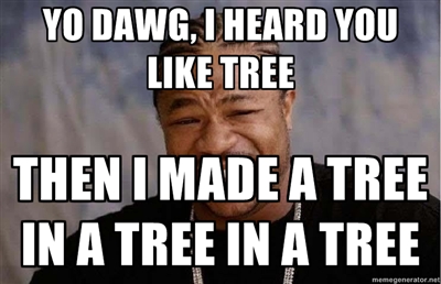
putStrLn "\nTree of Binary trees of Char binary trees:" print $ (treeFromList . map (treeFromList . map treeFromList)) [ ["YO","DAWG"] , ["I","HEARD"] , ["I","HEARD"] , ["YOU","LIKE","TREES"] ] :
print ( treeFromList ( map treeFromList [ map treeFromList ["YO","DAWG"] , map treeFromList ["I","HEARD"] , map treeFromList ["I","HEARD"] , map treeFromList ["YOU","LIKE","TREES"] ])) :
Binary tree of Binary trees of Char binary trees: < < < 'Y' : : : `--'O' : : `--< 'D' : : : |--'A' : : : `--'W' : : : `--'G' : |--< < 'I' : | : `--< 'H' : | : : |--'E' : | : : | `--'A' : | : : | `--'D' : | : : `--'R' : `--< < 'Y' : : : `--'O' : : : `--'U' : : `--< 'L' : : : `--'I' : : : |--'E' : : : `--'K' : : `--< 'T' : : : `--'R' : : : |--'E' : : : `--'S' , .
,
"I","HEARD" . () , Tree Eq .. , , . , !
02_Hard_Part/ 31_Trees.lhs
02_Hard_Part/ 40_Infinites_Structures.lhs
Haskell .
, Haskell . .
? Haskell-wiki:
( ) .(a+(b*c)),+,(b*c)
Haskell :
-- numbers = [1,2,..] numbers :: [Integer] numbers = 0:map (1+) numbers take' n [] = [] take' 0 l = [] take' n (x:xs) = x:take' (n-1) xs main = print $ take' 10 numbers .
How?
,
Haskell
[1..] ⇔ [1,2,3,4...] [1,3..] ⇔ [1,3,5,7,9,11...] .
take take' .02_Hard_Part/ 40_Infinites_Structures.lhs
02_Hard_Part/ 41_Infinites_Structures.lhs
, . :
nullTree = Node 0 nullTree nullTree . , , :
-- BinTree -- treeTakeDepth _ Empty = Empty treeTakeDepth 0 _ = Empty treeTakeDepth n (Node x left right) = let nl = treeTakeDepth (n-1) left nr = treeTakeDepth (n-1) right in Node x nl nr , :
main = print $ treeTakeDepth 4 nullTree , , :
< 0 : |-- 0 : | |-- 0 : | | |-- 0 : | | `-- 0 : | `-- 0 : | |-- 0 : | `-- 0 : `-- 0 : |-- 0 : | |-- 0 : | `-- 0 : `-- 0 : |-- 0 : `-- 0 , :
iTree = Node 0 (dec iTree) (inc iTree) where dec (Node xlr) = Node (x-1) (dec l) (dec r) inc (Node xlr) = Node (x+1) (inc l) (inc r) .
map , BinTree .:
-- Tree treeMap :: (a -> b) -> BinTree a -> BinTree b treeMap f Empty = Empty treeMap f (Node x left right) = Node (fx) (treeMap f left) (treeMap f right) : .
map , functor() fmap .:
infTreeTwo :: BinTree Int infTreeTwo = Node 0 (treeMap (\x -> x-1) infTreeTwo) (treeMap (\x -> x+1) infTreeTwo) main = print $ treeTakeDepth 4 infTreeTwo < 0 : |-- -1 : | |-- -2 : | | |-- -3 : | | `-- -1 : | `-- 0 : | |-- -1 : | `-- 1 : `-- 1 : |-- 0 : | |-- -1 : | `-- 1 : `-- 2 : |-- 1 : `-- 3 02_Hard_Part/ 41_Infinites_Structures.lhs
Source: https://habr.com/ru/post/152889/
All Articles