Method of geometric parallelism and some more about MPI
Hello, today I want to talk about the method of geometric parallelism for solving the two-dimensional heat equation. For clarity, some fragments will be implemented with the help of MPI in the C language. I will try not to repeat with this and this articles, and to tell something new.
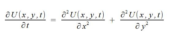
The two-dimensional heat conduction equation is given by the equation:
as well as initial conditions:
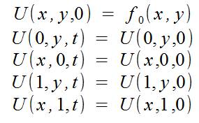
We also take into account that we calculate a limited area of space:

The result of our calculations should be a two-dimensional array containing the values of the function U in the nodes for a certain time value. You can solve the equation analytically, but this is not our option, and therefore we will solve this problem by a numerical method. For a numerical solution, we will make a discretization in time, and we will get a coordinate grid in space, and in time we will get a set of “layers”. For the calculation we will use the “cross” scheme.
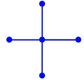
If we don’t go into the details of this scheme, then by the value at all points of the “cross” on some “time layer” we get the value at the central point on the “next time layer”. Moreover, the steps in time and coordinates must be consistent:
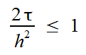
(hereinafter, the grid is fixed and the steps in spatial coordinates are h)
To save memory, you can store only two grids of X and Y, one for the current temporary layer and for the next temporary layer. In this case, after calculating the next temporary layer, this layer becomes the current one, and the values of the next temporary layer are written to the array of the last layer.
The method of geometric parallelism is used for problems in which it is possible to isolate a certain geometric regularity and use it to divide work between processors. In this task, the grid for limited space can be represented as:
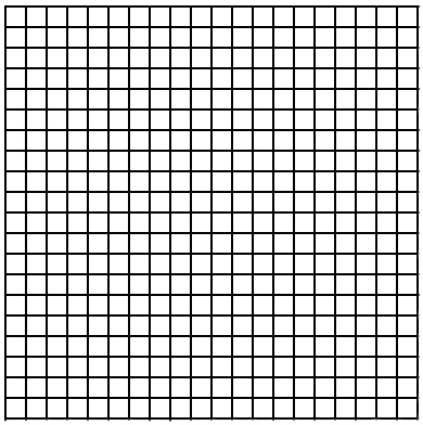
In this case, parallelism can be traced quite well and it is possible to divide the array into several, and each new one should be assigned to the performer.
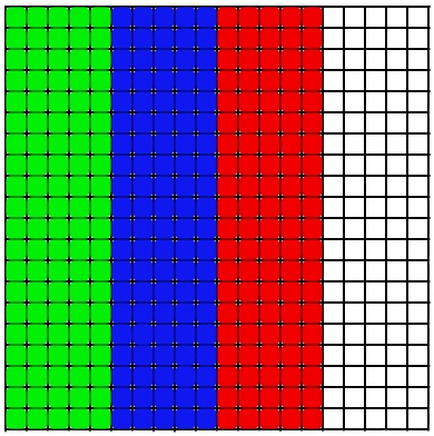
In general, it is possible to divide the array into horizontal stripes, this will not introduce fundamental differences for the method, but I’ll tell you about the implementation differences later. Thus, each performer will consider only his own part of the array.
If we return to the difference scheme, according to which we will calculate, it becomes clear that this is not the end. From the diagram it is clear that to calculate any element of the grid, we need to know the elements to the side of it in the previous layer. This means that we cannot calculate the outermost layer of the spatial grid (since there is not enough data), but if you look at the boundary conditions, you can see that the extreme elements are known from the conditions. But there is the problem of calculating the elements on the border of the performers. It is clear that in the process it will be necessary to transfer data between neighboring artists. This can be done in the form of a loop that passes over the element:
(more about the transfer of the elements can be found in the articles mentioned at the beginning)
This method is not effective because you have to establish many connections (this takes a lot of time). Our needs can satisfy the creation of a custom data type. In addition to creating custom structures, MPI can offer us several types of “masks” for data: MPI_Type_contiguous and MPI_Type_vector. The first of them creates a type that describes several elements arranged in a row in memory, and the second allows you to create a “template” by which “necessary” elements are selected from consecutively located elements in memory, then the “unnecessary” elements are skipped and the selection of the necessary ones is repeated. Their number is fixed.
If you send this type and specify the beginning of the array as * buf, you get:
+ 0 0
+ 0 0
+ 0 0
If you specify as * buf the second element of the array, we get:
0 + 0
0 + 0
0 + 0
')
So you can pass (and receive) only one column of the array, and in one call MPI_SEND:
If you arrange the performers' zones horizontally, you can use MPI_Type_contiguous or specify the required number of elements in MPI_Send, but this is, in my opinion, more beautiful.
Now we need to understand in what order to send these columns. The most obvious: let the performers in turn pass the desired column to the desired recipient. Then we get the following picture:
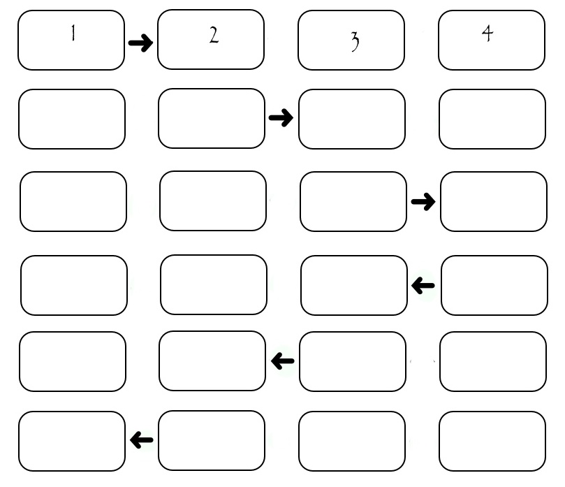
Although the illustration only shows the exchange between four performers, it can be calculated that if some SEND_TIME is spent on one transfer, then (2 * N-2) * SEND_TIME is needed to transfer all the columns. It can be seen that during the transmission of each column, only two performers "work", and the rest are idle. This is not good. Consider a slightly modified scheme: in it the performers are divided according to the "parity" of their number. First, all even pass the column to the performer with a large number, then all even pass the column to the performer with a lower number, then the performers with odd numbers come in the same way. Of course, all shipments occur only if there is someone to send to.
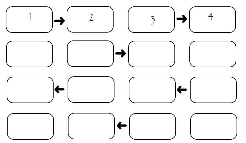
In this case, the transfer takes exactly 4 * SEND_TIME, regardless of the number of performers. On systems with a multitude of performers, this carries considerable superiority.
(In the pictures about the transfer there is a certain lie: the performer numbers start from zero, as in an array, and in the pictures they are numbered in the “usual” order: starting from the first. Ie, taking one from the number in the picture we get its number in the program)
Formulation of the problem
The two-dimensional heat conduction equation is given by the equation:
as well as initial conditions:
We also take into account that we calculate a limited area of space:
The result of our calculations should be a two-dimensional array containing the values of the function U in the nodes for a certain time value. You can solve the equation analytically, but this is not our option, and therefore we will solve this problem by a numerical method. For a numerical solution, we will make a discretization in time, and we will get a coordinate grid in space, and in time we will get a set of “layers”. For the calculation we will use the “cross” scheme.
If we don’t go into the details of this scheme, then by the value at all points of the “cross” on some “time layer” we get the value at the central point on the “next time layer”. Moreover, the steps in time and coordinates must be consistent:
(hereinafter, the grid is fixed and the steps in spatial coordinates are h)
To save memory, you can store only two grids of X and Y, one for the current temporary layer and for the next temporary layer. In this case, after calculating the next temporary layer, this layer becomes the current one, and the values of the next temporary layer are written to the array of the last layer.
Geometric parallelism method
The method of geometric parallelism is used for problems in which it is possible to isolate a certain geometric regularity and use it to divide work between processors. In this task, the grid for limited space can be represented as:
In this case, parallelism can be traced quite well and it is possible to divide the array into several, and each new one should be assigned to the performer.
In general, it is possible to divide the array into horizontal stripes, this will not introduce fundamental differences for the method, but I’ll tell you about the implementation differences later. Thus, each performer will consider only his own part of the array.
Underwater rocks
If we return to the difference scheme, according to which we will calculate, it becomes clear that this is not the end. From the diagram it is clear that to calculate any element of the grid, we need to know the elements to the side of it in the previous layer. This means that we cannot calculate the outermost layer of the spatial grid (since there is not enough data), but if you look at the boundary conditions, you can see that the extreme elements are known from the conditions. But there is the problem of calculating the elements on the border of the performers. It is clear that in the process it will be necessary to transfer data between neighboring artists. This can be done in the form of a loop that passes over the element:
for (int i = 0; i < N; i ++) { MPI_Send(*buf, 1, MPI_DOUBLE, toRank, MESSAGE_ID, MPI_COMM_WORLD); } (more about the transfer of the elements can be found in the articles mentioned at the beginning)
This method is not effective because you have to establish many connections (this takes a lot of time). Our needs can satisfy the creation of a custom data type. In addition to creating custom structures, MPI can offer us several types of “masks” for data: MPI_Type_contiguous and MPI_Type_vector. The first of them creates a type that describes several elements arranged in a row in memory, and the second allows you to create a “template” by which “necessary” elements are selected from consecutively located elements in memory, then the “unnecessary” elements are skipped and the selection of the necessary ones is repeated. Their number is fixed.
// - , // - "" // - , MPI_Datatype USER_Vector; MPI_Type_vector(N, 1, N, MPI_DOUBLE, &USER_Vector); // "" MPI_Type_commit(&USER_Vector); If you send this type and specify the beginning of the array as * buf, you get:
+ 0 0
+ 0 0
+ 0 0
If you specify as * buf the second element of the array, we get:
0 + 0
0 + 0
0 + 0
')
So you can pass (and receive) only one column of the array, and in one call MPI_SEND:
MPI_Send(*buf, 1, USER_Vector, (rank + 1), MESSAGE_ID, MPI_COMM_WORLD); If you arrange the performers' zones horizontally, you can use MPI_Type_contiguous or specify the required number of elements in MPI_Send, but this is, in my opinion, more beautiful.
Now we need to understand in what order to send these columns. The most obvious: let the performers in turn pass the desired column to the desired recipient. Then we get the following picture:
Although the illustration only shows the exchange between four performers, it can be calculated that if some SEND_TIME is spent on one transfer, then (2 * N-2) * SEND_TIME is needed to transfer all the columns. It can be seen that during the transmission of each column, only two performers "work", and the rest are idle. This is not good. Consider a slightly modified scheme: in it the performers are divided according to the "parity" of their number. First, all even pass the column to the performer with a large number, then all even pass the column to the performer with a lower number, then the performers with odd numbers come in the same way. Of course, all shipments occur only if there is someone to send to.
// EVEN_RIGHT, ODD_RIGHT, ODD_LEFT, EVEN_LEFT - // ( , ) const int ROOT = 0; if ((rank % 2) == 0) { if (rank != (size - 1)) MPI_Send(*buf, 1, USER_Vector, (rank + 1), EVEN_RIGHT, MPI_COMM_WORLD); if (rank != ROOT) MPI_Recv(*buf, 1, USER_Vector, (rank - 1), ODD_RIGHT, MPI_COMM_WORLD, &status); if (rank != (size - 1)) MPI_Recv(*buf, 1, USER_Vector, (rank + 1), ODD_LEFT, MPI_COMM_WORLD, &status); if (rank != ROOT) MPI_Send(*buf, 1, USER_Vector, (rank - 1), EVEN_LEFT, MPI_COMM_WORLD); } if ((rank % 2) == 1) { MPI_Recv(*buf, 1, USER_Vector, (rank - 1), EVEN_RIGHT, MPI_COMM_WORLD, &status); if (rank != (size - 1)) MPI_Send(*buf, 1, USER_Vector, (rank + 1), ODD_RIGHT, MPI_COMM_WORLD); MPI_Send(*buf, 1, USER_Vector, (rank - 1), ODD_LEFT, MPI_COMM_WORLD); if (rank != (size - 1)) MPI_Recv(*buf, 1, USER_Vector, (rank + 1), EVEN_LEFT, MPI_COMM_WORLD, &status); } In this case, the transfer takes exactly 4 * SEND_TIME, regardless of the number of performers. On systems with a multitude of performers, this carries considerable superiority.
(In the pictures about the transfer there is a certain lie: the performer numbers start from zero, as in an array, and in the pictures they are numbered in the “usual” order: starting from the first. Ie, taking one from the number in the picture we get its number in the program)
Source: https://habr.com/ru/post/151744/
All Articles