Fast blur according to Gauss
The Gaussian blur filter (commonly known as “gaussian blur” in Photoshop) is often used by itself or as part of other image processing algorithms. Next will be described a method that allows you to get a blur with a speed that does not depend on the blur radius using filters with infinite impulse response .
The description of the method is in English . But there is no information in Russian. In addition, I have made some changes.
So, let the original image be set by the brightness x ( m, n ). Gaussian blur with radius r is calculated by the formula
')
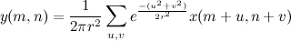
The summation limits for u and v can be chosen as plus or minus a few sigma, i.e. radii r , which gives the complexity of the algorithm of order O ( r 2 ) operations per pixel. For large r and multi-megapixel images, it's not too cool, is it?
The first acceleration gives the separability property of the Gaussian blur. That is, you can filter along the x axis for each row, filter the resulting image by y by each column and get the same result with complexity O ( r ) operations per pixel. Already better. We will also use this property, so further all the arguments will be for the one-dimensional case where you need to get y ( n ) with x ( n ).
This will help us filters with infinite impulse response. The idea of the filter is as follows: the values of y ( n ) are calculated recursively using the formula:
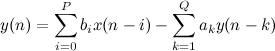
Where a k and b i are some of the pre-calculated coefficients, and y ( n ) and x ( n ) with n <0 are set to zero.
The part of the formula that depends on b i reduces to a simple convolution with a finite kernel . Since we want the filter to read faster, then we will look for our filter for the case P = 0, that is, considering a single coefficient b 0 .
Just in case, let me remind you that any linear filter (and the IIR filter is also linear) is completely characterized by its response to the delta function equal to 1 at point 0, and 0 at all other points. The part that depends on the coefficients a in response to such a function either disperses and goes to infinity (I would like to avoid this), or it will give us a beautiful decreasing tail. For example, like this:

Looks like gauss? Well, yes, something is already there, but somehow it looks kosoboko. Therefore, the idea of the algorithm will be as follows: we filter in one direction (in a cycle from 0 to n max ), and then the result is reversed (from n max to 0), with the same coefficients. Mathematically, you should get a strictly symmetric curve (therefore, it doesn’t matter if you first filter there and then back, or vice versa). A little running forward, that's what happens if you filter it in the reverse order:
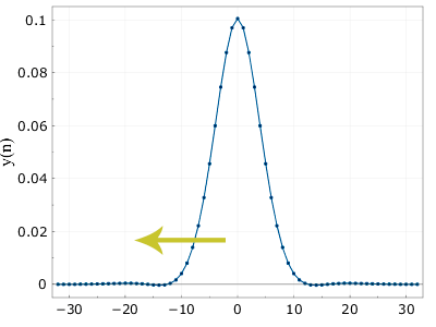
Here it is. Almost what we need. Almost, because in fact, of course, not really. The curve goes into the negative area a bit, and generally differs from the exact Gaussian. But for most applications, all this is quite acceptable, in addition, if you need to be considered quite certainly, you can increase the order of the Q filter.
So, it remains to calculate the filter coefficients a . Further, all the formulas will go for the case Q = 3.
In general, filters are studied using the so-called transfer function . Those interested can read what it is all about, and for a start, it will be enough for us to begin with that it simply exists and has certain properties. The general view of this function for a linear filter will be as follows:
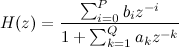
Or for our case Q = 3, P = 1:

Since there are polynomials in the numerator and denominator, they can be factorized. The numerator, in general, will give us zeros (in our case, there are no zeros), and the denominator will give us poles:
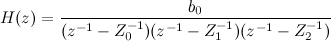
in our case, 1 / Z 0 , 1 / Z 1 , 1 / Z 2 . Note that the poles unambiguously determine the coefficients a k of our filter (all IIR filters are usually searched for precisely through the poles, and not directly). By the way, it is easier to get the coefficients by poles than vice versa (to do this, multiply the polynomials, and vice versa - to solve a power equation).
The most important theoretical postulate, which is useful to us: if the complex poles lie inside the unit circle, i.e. modulo less than one, (or, which is the same, the inverse values of Z 0 , Z 1 , Z 2 lie outside the unit circle), the filter will be stable, the result will not run away to infinity.
We also note that by calling arbitrary complex conjugate Z 0 , Z 1 and real Z 2 (again, all modulo more than one), we can build a filter on them. In the product, everything will turn into strictly real coefficients a .
The coefficient b 0 works like a filter's “volume coefficient”.
So, the task has been reduced to the definition of three coefficients Z 0 , Z 1 , Z 2 . Since, I repeat, two of them are complex conjugate, and the third is real, then you need to find the real and imaginary parts of the first, and the real part of the third. That is, three real numbers: real ( Z 0 ), im ( Z 0 ), Z 2
These three numbers must be expressed in terms of the filter radius we need. Note that in reality it makes sense to consider for r greater than or equal to two, for smaller values it is faster to filter by multiplication.
Then I went a little different way than in the work "Recursive Gaussian Derivative Filters". There they extended the case with r = 2 to all others, and I determined the best coefficients for all radii from 2 to 2048, with an exponential step. I wrote an optimization algorithm that looks for the closest curve using the method of minimizing the modulus of the maximum difference. An additional condition was the preservation of the total energy by the filter, i.e. so that the function x ( n ) = const goes into itself, which gives the condition
b 0 = 1- ( a 1 + a 2 + a 3 )
I tried different optimization algorithms, and the best ones produced a slightly modified genetic algorithm. (Perhaps, about the optimization, you can write a separate note).
Those interested can see the results on google spreadsheet .
It can be seen that for the case of r = 2, the results differ from those in the work. Why so, I can not say, while according to my calculations, my coefficients give a smaller, by 40 percent, error.
Then I used not the letter but the spirit of the article, and began to look for data as
real ( Z 0 ) = cos ( W ( r ) / r ) * e A ( r ) / r
im ( Z 0 ) = sin ( W ( r ) / r ) * e A ( r ) / r
Z 2 = e B ( r ) / r
Those. then you just need to pick up three similar functions, each of which tends in the limit in the constant. I was looking for a function in a relationship
( k 3 r 3 + k 2 r 2 + k 1 r + k 0 ) / r 3
and picked up the coefficients in the simplest way - just using Wolfram Mathematica . By the way, if you carefully study the graphics data from the tables, it is clear that the function has a somewhat sawtooth structure. Therefore, when approximating, we will lose a little in accuracy, but in fact just a little bit - the values from the table will give an error 10 percent less than those obtained by polynomials.
Here you go. For those who are already confused about what and what should be considered, I’ll give the final function code in C to calculate the coefficients:
Everything! Now, you need to write the code itself. Calculation, of course, needs to be made during float, but modern computers consider floating-point numbers (especially with sse) rather quickly. Programmers from Intel, by the way, have attended to the optimization of Gauss-IIR filters for the vector instructions of the processor have already written an entire article . True, they consider it a little differently, but the main optimization methods are described well.
In the end, you can give an example of what happened:
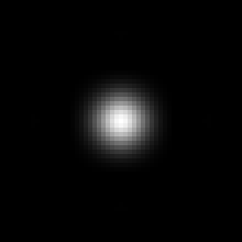
The picture is almost the same as “fair”. However, if you open it in Photoshop and study it carefully, you can find the difference.
PS This is true my first post on Habré, I could miss something. If you have questions, I will answer in the comments.
The description of the method is in English . But there is no information in Russian. In addition, I have made some changes.
So, let the original image be set by the brightness x ( m, n ). Gaussian blur with radius r is calculated by the formula
')
The summation limits for u and v can be chosen as plus or minus a few sigma, i.e. radii r , which gives the complexity of the algorithm of order O ( r 2 ) operations per pixel. For large r and multi-megapixel images, it's not too cool, is it?
The first acceleration gives the separability property of the Gaussian blur. That is, you can filter along the x axis for each row, filter the resulting image by y by each column and get the same result with complexity O ( r ) operations per pixel. Already better. We will also use this property, so further all the arguments will be for the one-dimensional case where you need to get y ( n ) with x ( n ).
This will help us filters with infinite impulse response. The idea of the filter is as follows: the values of y ( n ) are calculated recursively using the formula:
Where a k and b i are some of the pre-calculated coefficients, and y ( n ) and x ( n ) with n <0 are set to zero.
The part of the formula that depends on b i reduces to a simple convolution with a finite kernel . Since we want the filter to read faster, then we will look for our filter for the case P = 0, that is, considering a single coefficient b 0 .
Just in case, let me remind you that any linear filter (and the IIR filter is also linear) is completely characterized by its response to the delta function equal to 1 at point 0, and 0 at all other points. The part that depends on the coefficients a in response to such a function either disperses and goes to infinity (I would like to avoid this), or it will give us a beautiful decreasing tail. For example, like this:
Looks like gauss? Well, yes, something is already there, but somehow it looks kosoboko. Therefore, the idea of the algorithm will be as follows: we filter in one direction (in a cycle from 0 to n max ), and then the result is reversed (from n max to 0), with the same coefficients. Mathematically, you should get a strictly symmetric curve (therefore, it doesn’t matter if you first filter there and then back, or vice versa). A little running forward, that's what happens if you filter it in the reverse order:
Here it is. Almost what we need. Almost, because in fact, of course, not really. The curve goes into the negative area a bit, and generally differs from the exact Gaussian. But for most applications, all this is quite acceptable, in addition, if you need to be considered quite certainly, you can increase the order of the Q filter.
So, it remains to calculate the filter coefficients a . Further, all the formulas will go for the case Q = 3.
In general, filters are studied using the so-called transfer function . Those interested can read what it is all about, and for a start, it will be enough for us to begin with that it simply exists and has certain properties. The general view of this function for a linear filter will be as follows:
Or for our case Q = 3, P = 1:
Since there are polynomials in the numerator and denominator, they can be factorized. The numerator, in general, will give us zeros (in our case, there are no zeros), and the denominator will give us poles:
in our case, 1 / Z 0 , 1 / Z 1 , 1 / Z 2 . Note that the poles unambiguously determine the coefficients a k of our filter (all IIR filters are usually searched for precisely through the poles, and not directly). By the way, it is easier to get the coefficients by poles than vice versa (to do this, multiply the polynomials, and vice versa - to solve a power equation).
The most important theoretical postulate, which is useful to us: if the complex poles lie inside the unit circle, i.e. modulo less than one, (or, which is the same, the inverse values of Z 0 , Z 1 , Z 2 lie outside the unit circle), the filter will be stable, the result will not run away to infinity.
We also note that by calling arbitrary complex conjugate Z 0 , Z 1 and real Z 2 (again, all modulo more than one), we can build a filter on them. In the product, everything will turn into strictly real coefficients a .
The coefficient b 0 works like a filter's “volume coefficient”.
So, the task has been reduced to the definition of three coefficients Z 0 , Z 1 , Z 2 . Since, I repeat, two of them are complex conjugate, and the third is real, then you need to find the real and imaginary parts of the first, and the real part of the third. That is, three real numbers: real ( Z 0 ), im ( Z 0 ), Z 2
These three numbers must be expressed in terms of the filter radius we need. Note that in reality it makes sense to consider for r greater than or equal to two, for smaller values it is faster to filter by multiplication.
Then I went a little different way than in the work "Recursive Gaussian Derivative Filters". There they extended the case with r = 2 to all others, and I determined the best coefficients for all radii from 2 to 2048, with an exponential step. I wrote an optimization algorithm that looks for the closest curve using the method of minimizing the modulus of the maximum difference. An additional condition was the preservation of the total energy by the filter, i.e. so that the function x ( n ) = const goes into itself, which gives the condition
b 0 = 1- ( a 1 + a 2 + a 3 )
I tried different optimization algorithms, and the best ones produced a slightly modified genetic algorithm. (Perhaps, about the optimization, you can write a separate note).
Those interested can see the results on google spreadsheet .
It can be seen that for the case of r = 2, the results differ from those in the work. Why so, I can not say, while according to my calculations, my coefficients give a smaller, by 40 percent, error.
Then I used not the letter but the spirit of the article, and began to look for data as
real ( Z 0 ) = cos ( W ( r ) / r ) * e A ( r ) / r
im ( Z 0 ) = sin ( W ( r ) / r ) * e A ( r ) / r
Z 2 = e B ( r ) / r
Those. then you just need to pick up three similar functions, each of which tends in the limit in the constant. I was looking for a function in a relationship
( k 3 r 3 + k 2 r 2 + k 1 r + k 0 ) / r 3
and picked up the coefficients in the simplest way - just using Wolfram Mathematica . By the way, if you carefully study the graphics data from the tables, it is clear that the function has a somewhat sawtooth structure. Therefore, when approximating, we will lose a little in accuracy, but in fact just a little bit - the values from the table will give an error 10 percent less than those obtained by polynomials.
Here you go. For those who are already confused about what and what should be considered, I’ll give the final function code in C to calculate the coefficients:
int gaussCoef(double sigma, double a[3], double *b0) { double sigma_inv_4; sigma_inv_4 = sigma*sigma; sigma_inv_4 = 1.0/(sigma_inv_4*sigma_inv_4); double coef_A = sigma_inv_4*(sigma*(sigma*(sigma*1.1442707+0.0130625)-0.7500910)+0.2546730); double coef_W = sigma_inv_4*(sigma*(sigma*(sigma*1.3642870+0.0088755)-0.3255340)+0.3016210); double coef_B = sigma_inv_4*(sigma*(sigma*(sigma*1.2397166-0.0001644)-0.6363580)-0.0536068); double z0_abs = exp(coef_A); double z0_real = z0_abs*cos(coef_W); double z0_im = z0_abs*sin(coef_W); double z2 = exp(coef_B); double z0_abs_2 = z0_abs*z0_abs; a[2] = 1.0/(z2*z0_abs_2); a[0] = (z0_abs_2+2*z0_real*z2)*a[2]; a[1] = -(2*z0_real+z2)*a[2]; *b0 = 1.0 - a[0] - a[1] - a[2]; return 0; }; Everything! Now, you need to write the code itself. Calculation, of course, needs to be made during float, but modern computers consider floating-point numbers (especially with sse) rather quickly. Programmers from Intel, by the way, have attended to the optimization of Gauss-IIR filters for the vector instructions of the processor have already written an entire article . True, they consider it a little differently, but the main optimization methods are described well.
In the end, you can give an example of what happened:
The picture is almost the same as “fair”. However, if you open it in Photoshop and study it carefully, you can find the difference.
PS This is true my first post on Habré, I could miss something. If you have questions, I will answer in the comments.
Source: https://habr.com/ru/post/151157/
All Articles