Recommender systems: Bayes theorem and naive Bayes classifier
In this part we will not talk about recommender systems per se. Instead, we will separately concentrate on the main machine learning tool, the Bayes theorem, and consider one simple example of its application — the naive Bayes classifier. Disclaimer: I’m unlikely to tell something new to a reader familiar with the subject, let's talk mainly about the basic philosophy of machine learning.

Bayes' theorem either remembers or is trivial to deduce anyone who has passed even the most basic course of probability theory. Remember what conditional probability is x events provided y event? Directly by definition:
 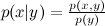 where
where  Is the joint probability of x and y , and p ( x ) and p ( y ) are the probabilities of each event separately. Hence, the joint probability can be expressed in two ways:
 .
.
Well, here's the Bayes theorem:

')
You probably think that I am making fun of you - how can a trivially tautological rewriting of the definition of conditional probability be the main tool of anything, especially such a big and nontrivial science as machine learning? However, let's begin to understand; at first, we simply rewrite the Bayes theorem in other notation (yes, I continue to mock):
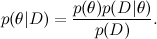
Now let's relate this to the typical machine learning task. Here D is the data, what we know, and θ are the parameters of the model that we want to train. For example, in the SVD model, the data are the ratings that users put on products, and the parameters of the model are the factors that we train for users and products.
Each of the probabilities also has its own meaning. - this is what we want to find, the probability distribution of the parameters of the model after we have taken into account the data; this is called posterior probability . This probability, as a rule, cannot be directly found, and this is precisely where the Bayes theorem is needed.
  - this is the so-called likelihood , the probability of the data, provided the model parameters are fixed; it is usually easy to find; in fact, the design of the model usually consists in setting the likelihood function. BUT
  - prior probability, it is a mathematical formalization of our intuition about the subject, a formalization of what we knew before, even before any experiments.
Here, probably, neither the time nor the place to go into it, but the merit of Reverend Thomas Bayes was, of course, not to rewrite the definition of conditional probability in two lines (there were no such definitions then), but just to put forward and develop such a view on the very concept of probability. Today, the “Bayesian approach” refers to the consideration of probabilities from the standpoint of “degrees of confidence” rather than the frictional (from the word frequency, not freak!) “Fraction of successful experiments when the total number of experiments is infinite”. In particular, this allows us to talk about the probabilities of one-time events - in fact there is no “number of experiments tending to infinity” for events like “Russia will become the world champion in 2018” or, closer to our subject, “Vasya will like the film” Tractor drivers ""; it's more like a dinosaur: either like it or not. Well, mathematics, of course, is always the same everywhere; Kolmogorov's axioms of probability don't care what they think of them.
To consolidate the traversed - a simple example. Consider the task of categorizing texts: for example, suppose that we are trying to sort the news flow based on an existing database with topics: sports, economics, culture ... We will use the so-called bag-of-words model: submit a document (multi) set words that it contains. As a result, each test case x takes values from a set of categories V and is described by attributes . We need to find the most likely value of this attribute, i.e.

By Bayes theorem,

Estimate easy: let's just estimate its frequency of occurrence. But appreciate the different
 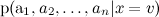 it won't work - there are too many of them - This is the probability of exactly such a set of words in messages on different topics. Obviously, such statistics take nowhere.
To cope with this, the naive Bayes classifier (the naive Bayes classifier — sometimes even called idiot's Bayes) implies conditional independence of attributes, subject to a given value of the objective function:

Now train the individual much simpler: it is enough to calculate the statistics of the occurrence of words in categories (there is one more detail that leads to two different variants of naive Bayes, but we will not go into details now).
Note that the naive Bayes classifier makes a damn strong assumption: in the text classification, we assume that different words in the text on the same topic appear independently of each other. This, of course, is complete nonsense - but, nevertheless, the results are quite decent. In fact, the naive Bayes classifier is much better than it seems. His estimates of probabilities are optimal, of course, only in the case of real independence; but the classifier itself is optimal in a much wider class of problems, and here's why. At first, attributes are, of course, dependent, but their dependency is the same for different classes and “mutually reduces” when evaluating probabilities. The grammatical and semantic dependencies between the words are the same in the text about football and in the text about Bayesian learning. Secondly, naive bayes are very bad for estimating probabilities, but as a classifier it is much better (usually, even if and
and  , naive Bayes will issue
  and
and  , but the classification will often be correct).
In the next series, we will complicate this example and consider the LDA model, which is able to highlight topics in the corpus of documents without any set of marked documents, moreover, so that one document can contain several topics, and also apply it to the task of recommendations.
Bayes' theorem either remembers or is trivial to deduce anyone who has passed even the most basic course of probability theory. Remember what conditional probability is
x events provided y event? Directly by definition: where Is the joint probability of x and y , and p ( x ) and p ( y ) are the probabilities of each event separately. Hence, the joint probability can be expressed in two ways: .Well, here's the Bayes theorem:
')
You probably think that I am making fun of you - how can a trivially tautological rewriting of the definition of conditional probability be the main tool of anything, especially such a big and nontrivial science as machine learning? However, let's begin to understand; at first, we simply rewrite the Bayes theorem in other notation (yes, I continue to mock):
Now let's relate this to the typical machine learning task. Here D is the data, what we know, and θ are the parameters of the model that we want to train. For example, in the SVD model, the data are the ratings that users put on products, and the parameters of the model are the factors that we train for users and products.
Each of the probabilities also has its own meaning.
- this is what we want to find, the probability distribution of the parameters of the model after we have taken into account the data; this is called posterior probability . This probability, as a rule, cannot be directly found, and this is precisely where the Bayes theorem is needed. - this is the so-called likelihood , the probability of the data, provided the model parameters are fixed; it is usually easy to find; in fact, the design of the model usually consists in setting the likelihood function. BUT - prior probability, it is a mathematical formalization of our intuition about the subject, a formalization of what we knew before, even before any experiments.Here, probably, neither the time nor the place to go into it, but the merit of Reverend Thomas Bayes was, of course, not to rewrite the definition of conditional probability in two lines (there were no such definitions then), but just to put forward and develop such a view on the very concept of probability. Today, the “Bayesian approach” refers to the consideration of probabilities from the standpoint of “degrees of confidence” rather than the frictional (from the word frequency, not freak!) “Fraction of successful experiments when the total number of experiments is infinite”. In particular, this allows us to talk about the probabilities of one-time events - in fact there is no “number of experiments tending to infinity” for events like “Russia will become the world champion in 2018” or, closer to our subject, “Vasya will like the film” Tractor drivers ""; it's more like a dinosaur: either like it or not. Well, mathematics, of course, is always the same everywhere; Kolmogorov's axioms of probability don't care what they think of them.
To consolidate the traversed - a simple example. Consider the task of categorizing texts: for example, suppose that we are trying to sort the news flow based on an existing database with topics: sports, economics, culture ... We will use the so-called bag-of-words model: submit a document (multi) set words that it contains. As a result, each test case x takes values from a set of categories V and is described by attributes
. We need to find the most likely value of this attribute, i.e.By Bayes theorem,
Estimate
easy: let's just estimate its frequency of occurrence. But appreciate the different it won't work - there are too many of them - This is the probability of exactly such a set of words in messages on different topics. Obviously, such statistics take nowhere.To cope with this, the naive Bayes classifier (the naive Bayes classifier — sometimes even called idiot's Bayes) implies conditional independence of attributes, subject to a given value of the objective function:
Now train the individual
much simpler: it is enough to calculate the statistics of the occurrence of words in categories (there is one more detail that leads to two different variants of naive Bayes, but we will not go into details now).Note that the naive Bayes classifier makes a damn strong assumption: in the text classification, we assume that different words in the text on the same topic appear independently of each other. This, of course, is complete nonsense - but, nevertheless, the results are quite decent. In fact, the naive Bayes classifier is much better than it seems. His estimates of probabilities are optimal, of course, only in the case of real independence; but the classifier itself is optimal in a much wider class of problems, and here's why. At first, attributes are, of course, dependent, but their dependency is the same for different classes and “mutually reduces” when evaluating probabilities. The grammatical and semantic dependencies between the words are the same in the text about football and in the text about Bayesian learning. Secondly, naive bayes are very bad for estimating probabilities, but as a classifier it is much better (usually, even if
and , naive Bayes will issue and , but the classification will often be correct).In the next series, we will complicate this example and consider the LDA model, which is able to highlight topics in the corpus of documents without any set of marked documents, moreover, so that one document can contain several topics, and also apply it to the task of recommendations.
Source: https://habr.com/ru/post/150207/
All Articles