An example of the practical use of copulas
In the previous article I explained the theoretical rationale for copulas. Since I myself was a student, I know that the best explanation of the theoretical apparatus can serve as an example of its practical application. Therefore, in this article I will try to show how copulas are used to model the interdependencies of several random variables.
As already mentioned, many copulas can reflect the dependence of not only two, but several quantities at once. This, of course, is good, but standard copulas imply some symmetry, that is, all pairwise dependencies will have the same pattern. Agree, this is not always true. To overcome this problem, an interesting and quite obvious (how much torment is hidden behind this word in mathematical analysis) was proposed - we break the joint copula into a set of two-dimensional copulas. We know that for n variables we will have pairwise interconnections. That is, we have to determine exactly how many pairwise copulas. We show that the joint distribution density of 4 values can be expressed as follows:
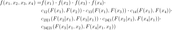
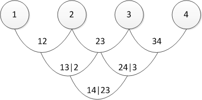
There are several ways to represent a partition, and the one mentioned above is called the canonical vine (I sincerely apologize, but I did not find an established translation of the “canonical vine” in the mathematical context, so I will use direct translation). Graphically, the last equation can be represented as follows:

Three trees describe the partition of a 4-dimensional copula. In the leftmost tree, the circles are marginal distributions, the arrows are two-dimensional copulas. Our task, as a person responsible for modeling, is to set all the "arrows", that is, to identify pairwise copulas and their parameters.
Now look at the formula of the D-shaped vine:
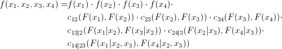
and its graphical representation
In fact, canonical and D-vines differ only in the order of determining pairwise dependencies. One may wonder - “how will I choose the order?” Or equivalent “and which vine should I choose?” I have an answer to this: in practice, they start with couples that show the greatest interconnection. The latter is determined by Kendall’s tau . Do not worry - everything will become clearer later when I show a direct practical example.
Once you have decided on the order of the definition of copulas, you need to understand which copulas to use for defining relationships (Gauss, Student, Gumbel, or some other). In principle, there is no exact scientific method. Someone is looking at the pairwise graphs of the distribution of the “archived” values and determine a copula by eye. Someone uses Chi-graphics ( it says how to use them ). A question of skill and an extensive field for research.
After we have decided which copulas to use in pairing, we need to determine their parameters. This is done by a numerical maximum likelihood method (numerical MLE) using the following algorithms:
These are algorithms for calculating the log-likelihood function, which, as is well known, must be maximized. This is a task for various optimization packages. It requires a small explanation of the variables used in the "code":
x is a set of “archived” data of size T by n, where x is limited on the interval (0,1).
v - matrix of size T on n-1 on n-1, where intermediate data will be loaded.
param - paired copula parameters, which we are looking for, maximizing the Log-likelihood.
L (x, v, param) =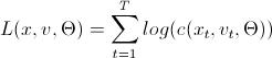
h (x, v, param) =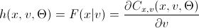
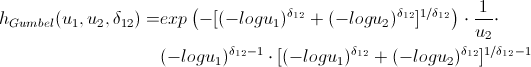
Fans of spoiling the paper with their calculations may not open the next spoiler, where I introduced the h-functions of the main copulas.
After we have found the parameters of our copulas, which maximize the logarithm likelihood function, we can proceed to the generation of random variables that have the same structure of interrelations as our initial data. For this, there are also algorithms:
You use the parameters that you obtained using the model estimation algorithms and generate n variables. You run this algorithm T times and get a matrix T by n, the data in which have the same pattern of interrelations as the original data. The only innovation compared with the previous algorithms is the inverse h-function (h_inv), which is the inverse function of the conditional distribution on the first variable.
Again, let me save you from lengthy calculations:
That's basically it. And now the promised ...
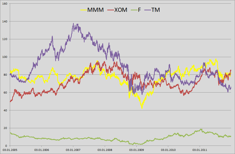
1. For example, I decided to play a small bank clerk, who was told to count the daily VaR in his portfolio. In the courtyard on January 1, 2012 and in my portfolio shares of 4 companies are in equal shares: 3M (MMM), Exxon Mobil (XOM), Ford Motors (F) and Toyota Motors (TM). Having played for the good i-tishniki, trying to get them to download price history from our server for the last 6 years, I realized that they had no time (January 1 outside, who generally works ???) and unloaded this information from Yaha's server. I took the price history by day for the period from January 3, 2005 to December 31, 2011. The result was a matrix of 1763 by 4.
2. Found logs: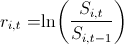 and built their pairwise distribution.
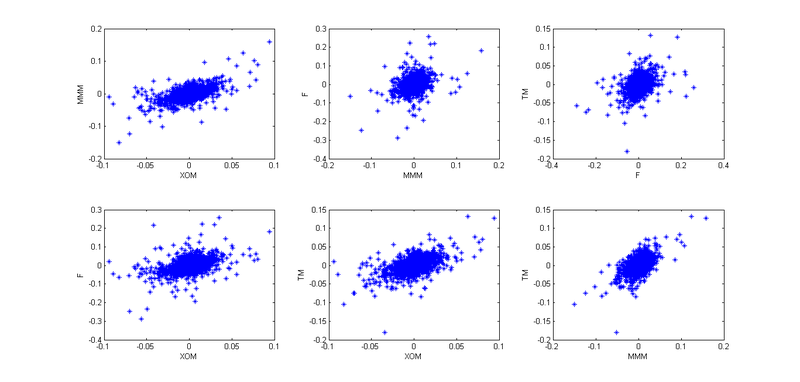
Well, to present the big picture.
3. Then I remembered the lectures on finance and how they hammered us - “guys, then the retrins are normally distributed - nonsense; in real life it's not like that. ” I wondered if I should use the assumption that the retrins are distributed along the NIG (Normal Inverse Gaussian). Studies show that this distribution fits well with empirical data. But I need to come up with a model for calculating VaR, and then test it on historical data. Any model that does not take into account the clustering of the second moment will show poor results. Then the idea came - I will use GARCH (1,1). The model well captures 3 and 4 moments of distribution, plus takes into account the volatility of the second moment. So, I decided that my retrins follow the following law . Here c is the historical average, z is a standard normally distributed random variable, and sigma follows its own law:
  .
.
4. So, now we need to take into account the interdependence of these four stocks. For a start, I used empirical copulas and plotted pairwise dependencies of “archived” observations:
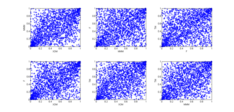
Considering that today is January 1, and I am a lazy little beast, I decided that all the patterns here are similar to Student’s copula, but in order to better convey interdependencies, I decided not to use the 4-dimensional copula, but to break it all into six 2-dimensional copulas.
5. In order to break into pair copulas, you need to choose the order of presentation - canonical or D-vine. For this, I counted tau kendall to determine the level of interdependence:
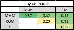
It is easy to see that MMM has the strongest ties with all other companies. This predetermines our choice of the vine - canonical. Why? Press PageUp a couple of times and look at its graphic display. In the first tree, all arrows emanate from the same node - it is our situation when one company has the strongest ties. If Kendall's high tau in the last table were on different lines and different columns, we would choose D-vine.
6. So, we have determined the order of presentation and all the necessary pairwise copulas - we can proceed to the evaluation of parameters. Applying the above algorithm for estimating the parameters of the canonical vine, I found all the necessary parameters.
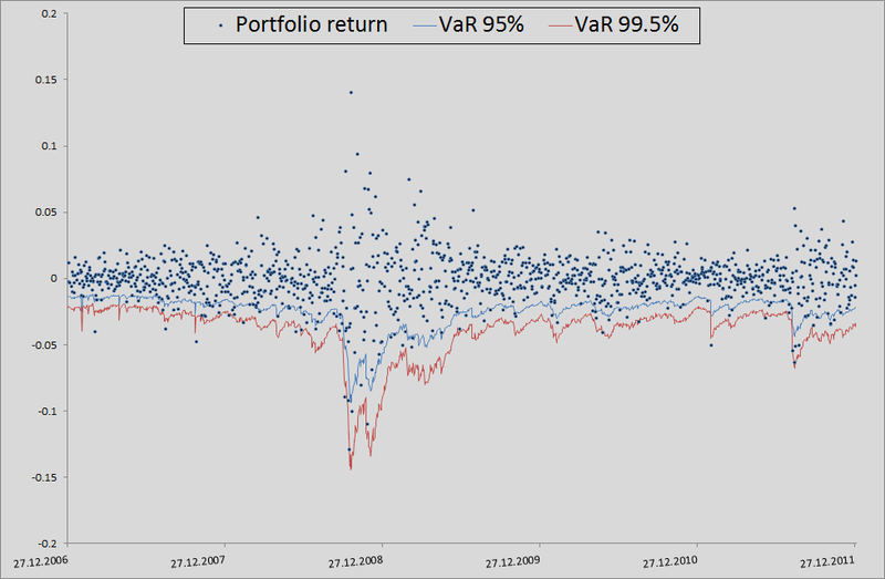
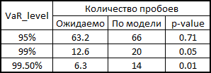
7. Here I will explain a little how this all happened in the context of backtesting. In order to check how much my model believes VaR is plausible, I would like to see how she coped in the past. For this, I gave her a small head start - 500 days and, starting from 501 days, I considered my risk metrics for the next day. Having copula parameters on my hands, I generated 10,000 quadruples of uniformly distributed values, received four quadrants of standard normally distributed quantities (noise) from them and substituted the formula of 3 points from this example into the calculation formula. There I also inserted a sigma forecast for the GARCH (1,1) model using data from previous days (this was done using a combination of matlabovskih functions ugarch and ugarchpred) and historical averages. Having thus received 10,000 quadruples of stocks, I received 10,000 retrans of my portfolio, taking the arithmetic mean of the stocks of stocks. (since we have equal shares and logs, we have the right to do so). Then sort and select the 50th, 100th, and 500th values for the 99.5%, 99%, and 95% thresholds, respectively. Having calculated the risk of the metrics for the remaining 1263 days, I received a beautiful graph and statistics of the level breakouts.
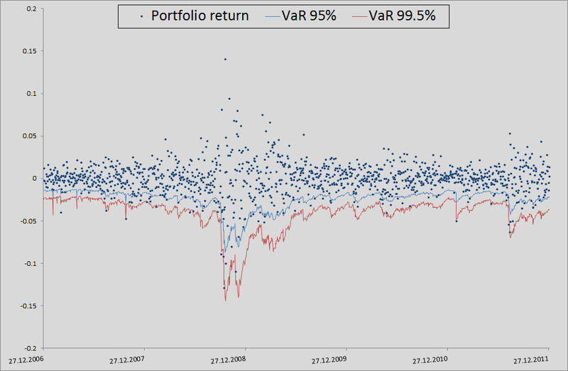
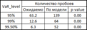
In principle, there is still room for growth in accuracy. But if we take as a benchmark model without taking into account interdependencies in general, then there are generally joints:
For honesty, you need to show how the model behaved if we used correlations and generated noises to calculate retterns from a multidimensional normal distribution:
As you can see, for VaR 95% this model is even better than ours. But the farther, the worse - as already mentioned, the normal distribution does not seize the tails.
In general, copulas can be used, but this must be done wisely. They provide more opportunities to take into account interdependencies, but, as with any exact model, you need to be careful here - you have the opportunity to miss the assumptions and get results worse than from the standard model.
PS Not once I noticed a stupid language behind me, so I will be glad if you point me to such moments in the text. I tried to express my thoughts as clearly as possible, but I do not always succeed.
Again a bit of theory
As already mentioned, many copulas can reflect the dependence of not only two, but several quantities at once. This, of course, is good, but standard copulas imply some symmetry, that is, all pairwise dependencies will have the same pattern. Agree, this is not always true. To overcome this problem, an interesting and quite obvious (how much torment is hidden behind this word in mathematical analysis) was proposed - we break the joint copula into a set of two-dimensional copulas. We know that for n variables we will have
pairwise interconnections. That is, we have to determine exactly how many pairwise copulas. We show that the joint distribution density of 4 values can be expressed as follows:slight evidence
To begin with, we recall that the distribution density of several quantities can be expressed as follows:

')
Also from the definition of a copula, we know that:

which in turn can be expressed as follows:

For the two-dimensional case, it will look like this:

And combining this with the very first formula, we get:

You can extend this example to the three-dimensional case:

and combining with the previous formula, we get:

Thus, we see that all elements from the first equation can be represented as a product of paired copulas and marginal density.
')
Also from the definition of a copula, we know that:
which in turn can be expressed as follows:
For the two-dimensional case, it will look like this:
And combining this with the very first formula, we get:
You can extend this example to the three-dimensional case:
and combining with the previous formula, we get:
Thus, we see that all elements from the first equation can be represented as a product of paired copulas and marginal density.
There are several ways to represent a partition, and the one mentioned above is called the canonical vine (I sincerely apologize, but I did not find an established translation of the “canonical vine” in the mathematical context, so I will use direct translation). Graphically, the last equation can be represented as follows:
Three trees describe the partition of a 4-dimensional copula. In the leftmost tree, the circles are marginal distributions, the arrows are two-dimensional copulas. Our task, as a person responsible for modeling, is to set all the "arrows", that is, to identify pairwise copulas and their parameters.
Now look at the formula of the D-shaped vine:
and its graphical representation
In fact, canonical and D-vines differ only in the order of determining pairwise dependencies. One may wonder - “how will I choose the order?” Or equivalent “and which vine should I choose?” I have an answer to this: in practice, they start with couples that show the greatest interconnection. The latter is determined by Kendall’s tau . Do not worry - everything will become clearer later when I show a direct practical example.
Once you have decided on the order of the definition of copulas, you need to understand which copulas to use for defining relationships (Gauss, Student, Gumbel, or some other). In principle, there is no exact scientific method. Someone is looking at the pairwise graphs of the distribution of the “archived” values and determine a copula by eye. Someone uses Chi-graphics ( it says how to use them ). A question of skill and an extensive field for research.
After we have decided which copulas to use in pairing, we need to determine their parameters. This is done by a numerical maximum likelihood method (numerical MLE) using the following algorithms:
Pseudocode for estimating the parameters of canonical vines
Log-likelihood=0; for i = 1:n v(0,i) = x(i) end for for j = 1:n-1 for i = 1:nj Log-likelihood = Log-likelihood + L(v(j-1,1), v(j-1,i+1), param(j,i)); end for if j == n then break end if for i = 1:nj v(j,i) = h(v(j-1,i+1), v(j-1,1), param(j,i)); end for end for Pseudocode for estimating the parameters of the D-vine
Log-likelihood=0; for i = 1:n v(0,i) = x(i); end for for j = 1:n-1 Log-likelihood = Log-likelihood + L(v(0,i),v(0,i+1), param(1,i)); end for v(1,1) = h(v(0,1),v(0,2), param(1,1)) for k = 1:n-3 v(1,2k) = h(v(0,k+2), v(0,k+1), param(1,k+1)); v(1,2k+1) = h(v(0,k+1), v(0,k+2), param(1,k+1)); end for v(1,2n-4) = h(v(0,n), v(0,n-1), param(1,n-1)); for j = 2:n-1 for i = 1:nj Log-likelihood = Log-likelihood + L(v(j-1,2i-1),v(j-1,2i), param(j,i)); end for if j == n-1 then break end if v(j,i) = h(v(j-1,1), v(j-1,2), param(j,1)); if n > 4 then for i = 1:nj-2 v(j,2i) = h(v(j-1,2i+2),v(j-1,2i+1),param(j,i+1)); v(j,2i+1) = h(v(j-1,2i+1),v(j-1,2i+2),param(j,i+1)); end for end if v(j,2n-2j-2) = h(v(j-1,2n-2j),v(j-1,2n-2j-1),param(j,nj)) end for These are algorithms for calculating the log-likelihood function, which, as is well known, must be maximized. This is a task for various optimization packages. It requires a small explanation of the variables used in the "code":
x is a set of “archived” data of size T by n, where x is limited on the interval (0,1).
v - matrix of size T on n-1 on n-1, where intermediate data will be loaded.
param - paired copula parameters, which we are looking for, maximizing the Log-likelihood.
L (x, v, param) =
h (x, v, param) =
Fans of spoiling the paper with their calculations may not open the next spoiler, where I introduced the h-functions of the main copulas.
h-functions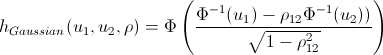

After we have found the parameters of our copulas, which maximize the logarithm likelihood function, we can proceed to the generation of random variables that have the same structure of interrelations as our initial data. For this, there are also algorithms:
Pseudocode for generating data on canonical vines
w = rand(n,1); % n x(1) = v(1,1) = w(1); for i = 2:n v(i,1) = w(i); for k = i-1:1 v(i,1) = h_inv(v(i,1), v(k,k), param(k,ik)); % , . end for x(i) = v(i,1); if i = n then break end if for j = 1:i-1 v(i,j+1) = h(v(i,j), v(j,j), param(j,ij)); end for end for Pseudocode to generate D-Vine data
w = rand(n,1); % n x(1) = v(1,1) = w(1); x(2) = v(2,1) = h_inv(w(2), v(1,1), param(1,1)); v(2,2) = h(v(1,1), v(2,1), param(1,1)); for i = 3:n v(i,1) = w(i); for k = i-1:2 v(i,1) = h_inv(v(i,1), v(i-1,2k-2), param(k,ik)); end for v(i,1) = h_inv(v(i,1), v(i-1,1), param(k,i-1)); x(i) = v(i,1); if i == n break end if v(i,2) = h(v(i-1,1), v(i,1), param(1,i-1)); v(i,3) = h(v(i,1), v(i-1,1), param(1,i-1)); if i>3 for j = 2:i-2 v(i,2j) = h(v(i-1,2j-2), v(i,2j-1), param(j,ij)); v(i,2j+1) = h(v(i,2j-1), v(i-1,2j-2), param(j,ij)); end for end if v(i,2i-2) = h(v(i-1,2i-4), v(i,2i-3), param(i-1,1)); end for You use the parameters that you obtained using the model estimation algorithms and generate n variables. You run this algorithm T times and get a matrix T by n, the data in which have the same pattern of interrelations as the original data. The only innovation compared with the previous algorithms is the inverse h-function (h_inv), which is the inverse function of the conditional distribution on the first variable.
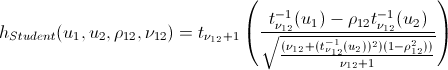
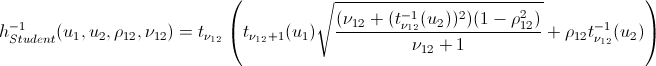
Again, let me save you from lengthy calculations:
inverse h-functions

That's basically it. And now the promised ...
Practical example
1. For example, I decided to play a small bank clerk, who was told to count the daily VaR in his portfolio. In the courtyard on January 1, 2012 and in my portfolio shares of 4 companies are in equal shares: 3M (MMM), Exxon Mobil (XOM), Ford Motors (F) and Toyota Motors (TM). Having played for the good i-tishniki, trying to get them to download price history from our server for the last 6 years, I realized that they had no time (January 1 outside, who generally works ???) and unloaded this information from Yaha's server. I took the price history by day for the period from January 3, 2005 to December 31, 2011. The result was a matrix of 1763 by 4.
2. Found logs:
and built their pairwise distribution.Well, to present the big picture.
3. Then I remembered the lectures on finance and how they hammered us - “guys, then the retrins are normally distributed - nonsense; in real life it's not like that. ” I wondered if I should use the assumption that the retrins are distributed along the NIG (Normal Inverse Gaussian). Studies show that this distribution fits well with empirical data. But I need to come up with a model for calculating VaR, and then test it on historical data. Any model that does not take into account the clustering of the second moment will show poor results. Then the idea came - I will use GARCH (1,1). The model well captures 3 and 4 moments of distribution, plus takes into account the volatility of the second moment. So, I decided that my retrins follow the following law
. Here c is the historical average, z is a standard normally distributed random variable, and sigma follows its own law: .4. So, now we need to take into account the interdependence of these four stocks. For a start, I used empirical copulas and plotted pairwise dependencies of “archived” observations:
Considering that today is January 1, and I am a lazy little beast, I decided that all the patterns here are similar to Student’s copula, but in order to better convey interdependencies, I decided not to use the 4-dimensional copula, but to break it all into six 2-dimensional copulas.
5. In order to break into pair copulas, you need to choose the order of presentation - canonical or D-vine. For this, I counted tau kendall to determine the level of interdependence:
It is easy to see that MMM has the strongest ties with all other companies. This predetermines our choice of the vine - canonical. Why? Press PageUp a couple of times and look at its graphic display. In the first tree, all arrows emanate from the same node - it is our situation when one company has the strongest ties. If Kendall's high tau in the last table were on different lines and different columns, we would choose D-vine.
6. So, we have determined the order of presentation and all the necessary pairwise copulas - we can proceed to the evaluation of parameters. Applying the above algorithm for estimating the parameters of the canonical vine, I found all the necessary parameters.
7. Here I will explain a little how this all happened in the context of backtesting. In order to check how much my model believes VaR is plausible, I would like to see how she coped in the past. For this, I gave her a small head start - 500 days and, starting from 501 days, I considered my risk metrics for the next day. Having copula parameters on my hands, I generated 10,000 quadruples of uniformly distributed values, received four quadrants of standard normally distributed quantities (noise) from them and substituted the formula of 3 points from this example into the calculation formula. There I also inserted a sigma forecast for the GARCH (1,1) model using data from previous days (this was done using a combination of matlabovskih functions ugarch and ugarchpred) and historical averages. Having thus received 10,000 quadruples of stocks, I received 10,000 retrans of my portfolio, taking the arithmetic mean of the stocks of stocks.
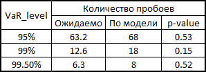
(since we have equal shares and logs, we have the right to do so). Then sort and select the 50th, 100th, and 500th values for the 99.5%, 99%, and 95% thresholds, respectively. Having calculated the risk of the metrics for the remaining 1263 days, I received a beautiful graph and statistics of the level breakouts.How to calculate p-value for VaR breakdown statistics
In 1995, Comrade Kupich proposed a formula for calculating the reliability of the VaR calculation model:

Here x is the number of breakdowns by model, T is the number of tests (we have = 1263), p is the expected share of breakdowns (in our case, 0.5%, 1% and 5%).
By the null hypothesis, this statistic has a chi-square distribution with one degree of freedom. Finding statistics, it is easy to count its p-value.
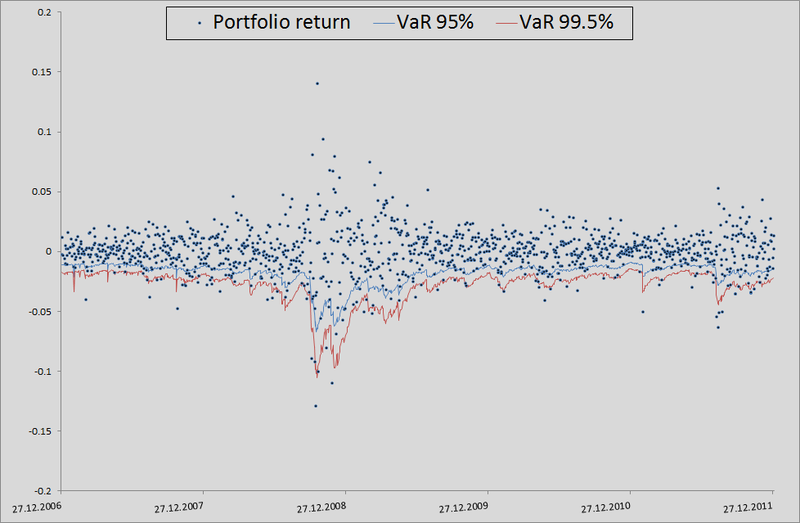
In principle, there is still room for growth in accuracy. But if we take as a benchmark model without taking into account interdependencies in general, then there are generally joints:
For honesty, you need to show how the model behaved if we used correlations and generated noises to calculate retterns from a multidimensional normal distribution:
As you can see, for VaR 95% this model is even better than ours. But the farther, the worse - as already mentioned, the normal distribution does not seize the tails.
In general, copulas can be used, but this must be done wisely. They provide more opportunities to take into account interdependencies, but, as with any exact model, you need to be careful here - you have the opportunity to miss the assumptions and get results worse than from the standard model.
PS Not once I noticed a stupid language behind me, so I will be glad if you point me to such moments in the text. I tried to express my thoughts as clearly as possible, but I do not always succeed.
Source: https://habr.com/ru/post/149543/
All Articles