Approximation of images by a genetic algorithm using EvoJ
In this article I will tell how you can apply a genetic algorithm to approximate images by polygons. As in my previous articles, for this purpose I will use my own EvoJ framework, which I have already written about here and here .

')
Following the traditional way of solving problems with the help of EvoJ, first we will choose how we describe the solutions for our problem. A straightforward solution would be to describe the approximation as a simple list of polygons:
This approach has the right to life, we will be able to pick up a satisfactory picture sooner or later. C is most likely late, since such an approach reduces the effectiveness of crossing good solutions. And that's why.
Imagine for simplicity the following picture.

Suppose we have two good solutions in the gene pool, each of which differs from the ideal one by one polygon.
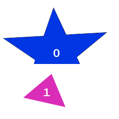
Pay attention to one feature: in both cases polygon number 0 ideally coincides with one of the image polygons, while the other lies somewhere to the side. It would be great to cross these two solutions so that, as a result, the first two polygons of both solutions turned out together, but this is not possible - EvoJ maps all variables to a byte array and, when crossed, works with bytes without changing their order.

The process of crossing over is explained in the following figure.

Thus, two elements with the same index can never be in the resulting solution.
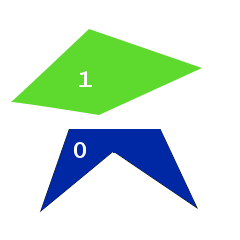
The result of crossing most likely will look like this:

That will greatly affect the effectiveness of crossing, significantly slowing down the evolution.
It is possible to get around the problem by sowing the original population “correctly” by evenly distributing polygons over the image area, so that the location of the polygon in the list is consistent with its geometric location in the figure. At the same time, it is necessary to limit the mutation so that the polygons cannot “crawl” too far.
A more advanced approach is to initially divide the image into cells, with each cell assigning its own list of polygons. In the form of a Java interface, this is described as:
The external list specifies rows of cells, the next nesting is columns, and finally, the internal list is polygons located in the corresponding cell. This approach automatically provides an approximate correspondence of the polygon position in a byte array and its geometrical location in the figure.
Each polygon will be described as:
Here the order property determines the global polygon rendering order. The color of the polygon is described as:
In other words, just as three components of color, those who wish can still add an alpha channel, however we will draw all polygons with 50% transparency, this will reduce the number of mutations that are indifferent. Assigning annotations here, I hope, obviously. If not, take a look at my previous articles, this question is dealt with there.
Polygon points will be described as:
In this case, the coordinates X and Y will be considered relative to the center of the cell to which the polygon belongs. Please note that annotations regulating the permissible values of variables are present only in the color description. This is due to the fact that the permissible values of the coordinates depend on the size of the image and on the configuration of the cells, and the permissible values of the color components are predefined things. In addition, the annotation on two internal lists in the
To set all the necessary parameters, we will use a mechanism called Detached Annotations.
So let's move on to programming. The sources used in this example can be found here . Much of the above code repeats what was written in my previous articles; a lot of things have nothing to do with the genetic algorithm as such. Therefore, I will focus on the key points, and the remaining parts are commented in the code.
Configuring EvoJ with Detached Annotations
Here we create a context -
Thus, the name of the
After the property name and
Annotation
The boundaries of the coordinates of points, the radius of their mutations, the limits of the values of the order property are set in a similar way.
Next, we use the completed context when creating the gene pool.
As a fitness function, we choose the sum of the squares of the deviations of the selected image from the original, with a minus sign - since the best solution corresponds to the smallest amount. The fitness function is implemented in the
As in the examples from previous articles, the class is inherited from the
and implements the abstract doCalcRating method as follows:
Here, the
The
As you can see, the function is rather trivial - it takes rasters of the original and freshly drawn images and compares them element by element, simultaneously adding (with a minus sign) the squares of differences.
In order to quickly achieve the result, it is necessary to choose the optimal mutation parameters:
The choice of strategy is not trivial. On the one hand, a strong mutation allows you to quickly cover the solution space and “grope” the global extremum, but on the other hand, it does not allow it to slide into it - solutions will constantly skip it. The long life of the solution insures against the deterioration of the fitness function value, but it slows down the overall progress and contributes to rolling into a local extremum instead of a global one. You also need to decide what to mutate with greater probability - the points of the polygons or their colors.
In addition, the chosen strategy exhausts itself after a while - the solutions found begin to oscillate around the extremum found, instead of slipping into it. To cope with this problem, strategies need to be changed. At the same time, the general idea is that the mutation level decreases with time, and the lifetime of successful solutions grows. The mutation strategies used in the example are chosen empirically.
Given all the above written, the main program cycle is as follows:
By running the program, after 15 minutes (depending on the power of your machine), you will find that the selected image already remotely resembles the original, and in an hour or two you will achieve a result close to that given at the beginning of the article.
Progress can be significantly accelerated by applying the following optimizations:
So, we looked at an example of how you can apply EvoJ to solve the problem of approximating an image. It is worth noting that the approximation of images by a genetic algorithm is more of an academic or aesthetic interest than a practical one, because a similar result can be achieved by other specially sharpened image vectoring algorithms.
Next time I will talk about the use of a genetic algorithm for generating design ideas.
UPD1: Since the link to the sources given in the text of the article is not striking, I duplicate it here http://evoj.sourceforge.net/static/demos/img-demo.rar
UPD2: At the request of workers, I cite slides from my first article
Choosing a method for describing the solution
')
Following the traditional way of solving problems with the help of EvoJ, first we will choose how we describe the solutions for our problem. A straightforward solution would be to describe the approximation as a simple list of polygons:
public interface PolyImage { List<Polygon> getCells(); } This approach has the right to life, we will be able to pick up a satisfactory picture sooner or later. C is most likely late, since such an approach reduces the effectiveness of crossing good solutions. And that's why.
Imagine for simplicity the following picture.
Suppose we have two good solutions in the gene pool, each of which differs from the ideal one by one polygon.
Pay attention to one feature: in both cases polygon number 0 ideally coincides with one of the image polygons, while the other lies somewhere to the side. It would be great to cross these two solutions so that, as a result, the first two polygons of both solutions turned out together, but this is not possible - EvoJ maps all variables to a byte array and, when crossed, works with bytes without changing their order.
The process of crossing over is explained in the following figure.
Thus, two elements with the same index can never be in the resulting solution.
The result of crossing most likely will look like this:
That will greatly affect the effectiveness of crossing, significantly slowing down the evolution.
It is possible to get around the problem by sowing the original population “correctly” by evenly distributing polygons over the image area, so that the location of the polygon in the list is consistent with its geometric location in the figure. At the same time, it is necessary to limit the mutation so that the polygons cannot “crawl” too far.
A more advanced approach is to initially divide the image into cells, with each cell assigning its own list of polygons. In the form of a Java interface, this is described as:
public interface PolyImage { Colour getBkColor(); List<List<List<Polygon>>> getCells(); } The external list specifies rows of cells, the next nesting is columns, and finally, the internal list is polygons located in the corresponding cell. This approach automatically provides an approximate correspondence of the polygon position in a byte array and its geometrical location in the figure.
Each polygon will be described as:
public interface Polygon { List<Point> getPoints(); Colour getColor(); int getOrder(); } Here the order property determines the global polygon rendering order. The color of the polygon is described as:
public interface Colour { @MutationRange("0.2") @Range(min = "0", max = "1", strict = "true") float getRed(); @MutationRange("0.2") @Range(min = "0", max = "1", strict = "true") float getGreen(); @MutationRange("0.2") @Range(min = "0", max = "1", strict = "true") float getBlue(); void setRed(float red); void setGreen(float green); void setBlue(float blue); } In other words, just as three components of color, those who wish can still add an alpha channel, however we will draw all polygons with 50% transparency, this will reduce the number of mutations that are indifferent. Assigning annotations here, I hope, obviously. If not, take a look at my previous articles, this question is dealt with there.
Polygon points will be described as:
public interface Point { int getX(); int getY(); } In this case, the coordinates X and Y will be considered relative to the center of the cell to which the polygon belongs. Please note that annotations regulating the permissible values of variables are present only in the color description. This is due to the fact that the permissible values of the coordinates depend on the size of the image and on the configuration of the cells, and the permissible values of the color components are predefined things. In addition, the annotation on two internal lists in the
PolyImage interface cannot be hanged at all.To set all the necessary parameters, we will use a mechanism called Detached Annotations.
So let's move on to programming. The sources used in this example can be found here . Much of the above code repeats what was written in my previous articles; a lot of things have nothing to do with the genetic algorithm as such. Therefore, I will focus on the key points, and the remaining parts are commented in the code.
Configuring EvoJ with Detached Annotations
final HashMap<String, String> context = new HashMap<String, String>(); context.put("cells@Length", ROWS.toString()); context.put("cells.item@Length", COLUMNS.toString()); context.put("cells.item.item@Length", POLYGONS_PER_CELL.toString()); context.put("cells.item.item.item.points@Length", "6"); context.put("cells.item.item.item.points.item.x@StrictRange", "true"); context.put("cells.item.item.item.points.item.x@Min", String.valueOf(-widthRadius)); context.put("cells.item.item.item.points.item.x@Max", String.valueOf(widthRadius)); context.put("cells.item.item.item.points.item.x@MutationRange", "20"); context.put("cells.item.item.item.points.item.y@StrictRange", "true"); context.put("cells.item.item.item.points.item.y@Min", String.valueOf(-heightRadius)); context.put("cells.item.item.item.points.item.y@Max", String.valueOf(heightRadius)); context.put("cells.item.item.item.points.item.y@MutationRange", "20"); context.put("cells.item.item.item.order@Min", "0"); context.put("cells.item.item.item.order@Max", "1000"); Here we create a context -
Map similar to the properties file, where the name of the property corresponds to the path to the property of the object in a notation similar to the one accepted in BeanUtils , except that the list items are indicated by the keyword item .Thus, the name of the
cells describes the cells property of our root PolyImage interface. And the line cells.item are the elements of this list, which in turn are the lists described by the line cells.item.item , and so on.After the property name and
@ sign, the name of the detached annotation is indicated, which is similar to the name of a regular annotation. It is mandatory to specify the length of the list so that EvoJ knows how much space to reserve in the byte array.Annotation
cells.item.item.item.points@Length sets the number of points in a polygon (follow the path — the cells property, three nested lists, the points property of the elements of the nested list itself.The boundaries of the coordinates of points, the radius of their mutations, the limits of the values of the order property are set in a similar way.
Next, we use the completed context when creating the gene pool.
Creating a fitness function
As a fitness function, we choose the sum of the squares of the deviations of the selected image from the original, with a minus sign - since the best solution corresponds to the smallest amount. The fitness function is implemented in the
ImageRating class, ImageRating 's focus on its key points.As in the examples from previous articles, the class is inherited from the
AbstractSimpleRating helper-class: public class ImageRating extends AbstractSimpleRating<PolyImage> and implements the abstract doCalcRating method as follows:
@Override protected Comparable doCalcRating(PolyImage solution) { BufferedImage tmp = drawImage(solution); return compareImages(originalImage, tmp); } Here, the
drawImage function trivially drawImage all polygons according to their cell, order, color, and so on. We will not dwell on it in detail - it does not contain anything related to the genetic algorithm.The
compareImages function performs pixel-by-pixel comparison of images. Consider it a little closer. private Comparable compareImages(BufferedImage originalImage, BufferedImage tmp) { long result = 0; int[] originalPixels = originalImage.getRaster().getPixels(0, 0, originalImage.getWidth(), originalImage.getHeight(), (int[]) null); int[] tmpPixels = tmp.getRaster().getPixels(0, 0, tmp.getWidth(), tmp.getHeight(), (int[]) null); for (int i = 0; i < originalPixels.length; i++) { long d = originalPixels[i] - tmpPixels[i]; result -= d * d; } return result; } As you can see, the function is rather trivial - it takes rasters of the original and freshly drawn images and compares them element by element, simultaneously adding (with a minus sign) the squares of differences.
Iteration
In order to quickly achieve the result, it is necessary to choose the optimal mutation parameters:
- the likelihood that the decision will generally undergo a mutation
- probability of mutation of each variable inside the solution
- radius of change - the maximum distance that a point can move during a mutation
- solution lifetime (not entirely related to mutation, but also affects the rate of convergence)
The choice of strategy is not trivial. On the one hand, a strong mutation allows you to quickly cover the solution space and “grope” the global extremum, but on the other hand, it does not allow it to slide into it - solutions will constantly skip it. The long life of the solution insures against the deterioration of the fitness function value, but it slows down the overall progress and contributes to rolling into a local extremum instead of a global one. You also need to decide what to mutate with greater probability - the points of the polygons or their colors.
In addition, the chosen strategy exhausts itself after a while - the solutions found begin to oscillate around the extremum found, instead of slipping into it. To cope with this problem, strategies need to be changed. At the same time, the general idea is that the mutation level decreases with time, and the lifetime of successful solutions grows. The mutation strategies used in the example are chosen empirically.
Given all the above written, the main program cycle is as follows:
- perform 10 iterations of the genetic algorithm
- take the value of the fitness function from the best solution
- determine whether it is time to change the strategy
- change strategy if necessary
- save picture to temporary file
- update ui
By running the program, after 15 minutes (depending on the power of your machine), you will find that the selected image already remotely resembles the original, and in an hour or two you will achieve a result close to that given at the beginning of the article.
Further improvement of the algorithm
Progress can be significantly accelerated by applying the following optimizations:
- approximation is performed in Lab space instead of RGB; it is characterized by the fact that the Cartesian distance between points in the color space is approximately consistent with the perceived difference. The number of iterations per second does not add it, but it will direct the evolution in the right direction.
- create a mask of the importance of image areas - a black and white image with selected areas of interest, which can then be used when calculating the fitness function; this will allow the evolution to focus on what is really interesting.
- for images use VolatileImage. On my machine, drawing on VolatileImage is 10 times faster than drawing on BufferedImage. True, then the result has to be converted to BufferedImage anyway in order to get the colors of the pixels, this leads to a significant drop in performance, but still the final result is 3 times better than just drawing polygons on BufferedImage.
- select the optimal mutation parameters at different stages. The task is not simple, but even here a genetic algorithm can help. I conducted experiments where the variables were mutation parameters, and the fitness function was the average rate of error reduction per 100 iterations. The results are encouraging, but to solve this problem requires significant computational power. Probably I in one of the following articles I will sort this problem closer.
- start several independent gene pools and make an evolution in them independently, at certain intervals, cross each other individuals from different gene pools. Such an approach is called the island model of the GA, i.e., evolution seems to take place on islands isolated from each other, crosses between individuals from different islands are extremely rare.
- sow the image with polygons gradually: first place 1-2 polygons in each cell, allow them to “spread out”, then add another 1-2 polygons to the places where the image deviates from the original the greatest and only evolve newly added polygons, repeat this until the limit of the number of polygons in the cell is reached, and then start the evolution across the entire image, as described in the article above. This approach leads to the most accurate close approximations.
Afterword
So, we looked at an example of how you can apply EvoJ to solve the problem of approximating an image. It is worth noting that the approximation of images by a genetic algorithm is more of an academic or aesthetic interest than a practical one, because a similar result can be achieved by other specially sharpened image vectoring algorithms.
Next time I will talk about the use of a genetic algorithm for generating design ideas.
UPD1: Since the link to the sources given in the text of the article is not striking, I duplicate it here http://evoj.sourceforge.net/static/demos/img-demo.rar
UPD2: At the request of workers, I cite slides from my first article
| Source image | Matched image |
|---|---|
 |  |
 |  |
Source: https://habr.com/ru/post/149161/
All Articles