How I bought an apartment
I wanted to write an article about linear regression, but then I thought, well, well, better buy an apartment. And he went to look for what they offer. A offer, as it turned out, a lot of things. More than 500 apartments fell into the price range that suits me. And what, I now see all this? Well nooo, I am a programmer in the end or not a programmer. We must somehow automate this matter.
Before you decide something, it would be nice to look at the big picture, to see some sort of squeeze from the data. And for this, data must first be collected. I was interested in apartments in Minsk up to $ 60k (I hope the Muscovites did not choke on saliva, having learned that for such money to actually buy an apartment?). Google immediately issued several websites about real estate, among which the largest number of search settings I needed turned out to be on irr.by. The design of him, of course, is not a fountain, but I, too, am not a blonde girl, to choose a real estate site by color. And the data in the form of HTML-pages in any case did not suit me.
For a couple of hours, I threw in the parser, which took the search string as input, ran through the first 5 pages of results and collected the parameters of interest to me. And I was interested in the following things:
')
The only thing that raised questions was the distance to the metro. Real estate sites usually do not provide this information. There is only the name of the street, the house number and the nearest station, but how many times to go there is not a word about it. Fortunately, it turned out that the problem of determining the coordinates at an address is not new, and the corresponding process is called geocoding , and the Babla Corporation even provides a free service for this good deed. After half an hour of programming with a break for coffee and cookies, the module for determining the distance to the metro at the address was ready. (It should be noted that the results were very accurate - out of about 50 verified addresses, only 2 indicated the street, but not the house; the rest were completely correct. You should also pay attention to the fact that the service is better not to DDOS - if you don’t small breaks between requests, errors may occur.)
Since sellers are far from always carefully and accurately filling in the fields for describing an apartment, the data were incomplete. In an amicable way, the blank fields had to be marked as NA (Not Available) and passed them on in this form. But it was in the evening, and there was still something to do, so I decided to follow a simplified scheme and, at the data collection stage, to score the default values. In the absence of information about the year of construction, I scored 1980 (respectively, age - 32 years), the distance to the metro - 2000 meters, floor - 4, number of floors - 7. Very simple and almost at random. The number of rooms, the area and the price were obligatory parameters, and in their absence the apartment was simply discarded (although in the end there was not a single case of the absence of at least one of these parameters).
Separately, you need to tell about the type of bathroom. Anticipating numerical calculations, I realized that working with common / separate values was much more difficult than with numbers, so I had to create 2 separate variables, one for each type. Moreover, if one variable was equal to 1, then the second was necessarily equal to 0. In statistics, this is called fictitious or indicator variables .
But enough about the toilets, it's time to look at the data.
One of the most popular data analysis tools is the R project . R is a development environment and a programming language with extensive capabilities for manipulating and visualizing data, as well as statistical analysis and machine learning. There are several development environments for easy editing of scripts, such as RStudio and Emacs plugin , but for most tasks a regular console is sufficient. All this is cross-platform and completely free, that is, in vain. R undoubtedly deserves a separate detailed article, here I will limit myself to a description of the functions and constructions of the language that I will use directly.
The ad parser, which I described above, saved the data as a CSV file on disk. To load it into R, just call the following function:
, , `<-`. `=`, . , , .. :
dat ( «data» ) `data.frame`. — R , , , `_` C `-` Lisp ( , , , - - , ). : , , . , price (6- ) :
:
:
, R . plot(). , 2 ( , ) (scatter plot). plot() , R :
, . :
:
! 3- 4- ! . . dist_to_subway :
, 4 (`dat[dat$room_no == 4, ]`), (`$dist_to_subway`). — . , (2000 ), . , . , - , . . . , 1-, 3- 4-, ( ) URL ( ). , , , restroom_sep restroom_com , .
: , /.
, , . cor(), , , , ( ):
, (> 0.6) , . 2- — living_space kitchen_space — total_space.
, . , : (, ) (, ), . , :

, . , , , , - .
, , - :


, , , , — , , .
, , , . , «». . , , , . — , , , .
-, ? ? , , :
? , . y x, ( «») , .
, 2 ? :
n , :
() :
,
~ , lm() «». , , R , , . ( ) , (age, balcony, etc.). :
, ( , ).
? , , :
. predict(), , «» :
:

, — . — . , . , . .
.
, 343- ( ) 20% ( $10k, ), 233 — 15% .. , ?
: , , , .
, , 8 . : , , , . , . . -, , . -, , . , -, .
. . , ?..
:
1. . flatparser.jar ( , View Raw) README.
2. Coursera, , , .
Data collection
Before you decide something, it would be nice to look at the big picture, to see some sort of squeeze from the data. And for this, data must first be collected. I was interested in apartments in Minsk up to $ 60k (I hope the Muscovites did not choke on saliva, having learned that for such money to actually buy an apartment?). Google immediately issued several websites about real estate, among which the largest number of search settings I needed turned out to be on irr.by. The design of him, of course, is not a fountain, but I, too, am not a blonde girl, to choose a real estate site by color. And the data in the form of HTML-pages in any case did not suit me.
For a couple of hours, I threw in the parser, which took the search string as input, ran through the first 5 pages of results and collected the parameters of interest to me. And I was interested in the following things:
- price (hereinafter - the variable price)
- age
- distance to metro (dist_to_subway)
- floor (storey) and storey of the house (storey_no)
- availability of a balcony or loggia (balcony)
- total (total_space) and living area (living_space), as well as kitchen area (kitchen_space)
- number of separate rooms (room_no)
- bathroom type (restroom_com for general, restroom_sep for separate)
')
The only thing that raised questions was the distance to the metro. Real estate sites usually do not provide this information. There is only the name of the street, the house number and the nearest station, but how many times to go there is not a word about it. Fortunately, it turned out that the problem of determining the coordinates at an address is not new, and the corresponding process is called geocoding , and the Babla Corporation even provides a free service for this good deed. After half an hour of programming with a break for coffee and cookies, the module for determining the distance to the metro at the address was ready. (It should be noted that the results were very accurate - out of about 50 verified addresses, only 2 indicated the street, but not the house; the rest were completely correct. You should also pay attention to the fact that the service is better not to DDOS - if you don’t small breaks between requests, errors may occur.)
Since sellers are far from always carefully and accurately filling in the fields for describing an apartment, the data were incomplete. In an amicable way, the blank fields had to be marked as NA (Not Available) and passed them on in this form. But it was in the evening, and there was still something to do, so I decided to follow a simplified scheme and, at the data collection stage, to score the default values. In the absence of information about the year of construction, I scored 1980 (respectively, age - 32 years), the distance to the metro - 2000 meters, floor - 4, number of floors - 7. Very simple and almost at random. The number of rooms, the area and the price were obligatory parameters, and in their absence the apartment was simply discarded (although in the end there was not a single case of the absence of at least one of these parameters).
Separately, you need to tell about the type of bathroom. Anticipating numerical calculations, I realized that working with common / separate values was much more difficult than with numbers, so I had to create 2 separate variables, one for each type. Moreover, if one variable was equal to 1, then the second was necessarily equal to 0. In statistics, this is called fictitious or indicator variables .
But enough about the toilets, it's time to look at the data.
First look at the data
One of the most popular data analysis tools is the R project . R is a development environment and a programming language with extensive capabilities for manipulating and visualizing data, as well as statistical analysis and machine learning. There are several development environments for easy editing of scripts, such as RStudio and Emacs plugin , but for most tasks a regular console is sufficient. All this is cross-platform and completely free, that is, in vain. R undoubtedly deserves a separate detailed article, here I will limit myself to a description of the functions and constructions of the language that I will use directly.
The ad parser, which I described above, saved the data as a CSV file on disk. To load it into R, just call the following function:
> dat <- read.csv("/path/to/dataset.csv")
, , `<-`. `=`, . , , .. :
> read.csv("/path/to/dataset.csv") -> dat
dat ( «data» ) `data.frame`. — R , , , `_` C `-` Lisp ( , , , - - , ). : , , . , price (6- ) :
> dat[6]
> dat["price"] # - dat$price
:
> dat[3, 6] # 3 6
:
  > dat[1:10, 1:6]     # ,    10    6
  > dat[1:10, c(3, 5)] #  10    3  5
  > dat[, 6]           #   6-  ( dat[6])
  > dat[, -6]          #    ,  6
  > dat[,]             #     ( dat)
, R . plot(). , 2 ( , ) (scatter plot). plot() , R :
> ?plot
, . :
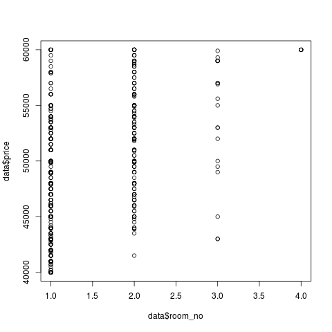
> plot(dat$room_no, dat$price)
:
! 3- 4- ! . . dist_to_subway :
  > dat[dat$room_no == 4, ]$dist_to_subway
   [1] 2000.000 2000.000 2000.000 2000.000 4305.613
, 4 (`dat[dat$room_no == 4, ]`), (`$dist_to_subway`). — . , (2000 ), . , . , - , . . . , 1-, 3- 4-, ( ) URL ( ). , , , restroom_sep restroom_com , .
> dat2 <- dat[dat$room_no == 2, -(7, 8, 9, 13)]
: , /.
, , . cor(), , , , ( ):
  > cor(dat2)
                       age     balcony dist_to_subway kitchen_space living_space
 age             1.0000000  0.23339483     0.23677636   -0.30167358  -0.18938523
 balcony         0.2333948  1.00000000    -0.06881481    0.05694279  -0.03505876
 dist_to_subway  0.2367764 -0.06881481     1.00000000    0.22700865  -0.21201038
 kitchen_space  -0.3016736  0.05694279     0.22700865    1.00000000   0.10018058
 living_space   -0.1893852 -0.03505876    -0.21201038    0.10018058   1.00000000
 price          -0.2246434  0.18848129    -0.11713353    0.35152990   0.22979332
 storey         -0.1740015  0.12504337    -0.03107719    0.22760853   0.09702503
 storey_no      -0.4683041 -0.28689325    -0.15872038    0.10098619   0.02122686
 total_space    -0.3732784  0.02748897     0.03466465    0.62723545   0.61874577
                     price      storey   storey_no total_space
 age            -0.2246434 -0.17400151 -0.46830412 -0.37327839
 balcony         0.1884813  0.12504337 -0.28689325  0.02748897
 dist_to_subway -0.1171335 -0.03107719 -0.15872038  0.03466465
 kitchen_space   0.3515299  0.22760853  0.10098619  0.62723545
 living_space    0.2297933  0.09702503  0.02122686  0.61874577
 price           1.0000000  0.35325897  0.24603010  0.51735302
 storey          0.3532590  1.00000000  0.26811766  0.18082811
 storey_no       0.2460301  0.26811766  1.00000000  0.14940533
 total_space     0.5173530  0.18082811  0.14940533  1.00000000
, (> 0.6) , . 2- — living_space kitchen_space — total_space.
, . , : (, ) (, ), . , :
> plot(dat2$dist_to_subway, dat2$price)
, . , , , , - .
, , - :
> plot(dat2$dist_to_subway, dat2$price)
> plot(dat2$age, dat2$price)
, , , , — , , .
, , , . , «». . , , , . — , , , .
-, ? ? , , :
y = k * x + b
? , . y x, ( «») , .
k X, b — Y ., 2 ? :
z = k1 * x + k2 * y + b
n , :
h(X) = k0 + k1 * x1 + k2 * x2 + ... + kn * xn
x1..xn — , h(X) — X.() :
price = k0 + k1 * age + k2 * balcony + k3 * dist_to_subway + k4 * storey + k5 * storey_no + k6 * total_space
,
k0..k6 ! , , ? . , (, ) , . , R, lm() ( Linear Model): > model <- lm(price ~ age + balcony + dist_to_subway + storey + storey_no + total_space, data = dat2)
~ , lm() «». , , R , , . ( ) , (age, balcony, etc.). :
> model <- lm(price ~ ., data = dat2)
, ( , ).
? , , :
  > coef(model)
     (Intercept)            age        balcony dist_to_subway         storey
   21601.0057018     31.7479138   1981.3750585     -0.3962895    529.9350262
       storey_no    total_space
     594.3711746    523.7914531
(Intercept) k0 (, , , , , ). . total_space ( , , — intercept). 2 , 40 . , , . , , . , . . -, , , . -, , , 32- ( ) . -, , , .. predict(), , «» :
> predicted.cost <- predict(model, dat2)
:
  > actual.price <- dat2$price         #
  > plot(predicted.cost, actual.price) #   vs.
  > par(new=TRUE, col="red")           #  :     ,
  > dependency <- lm(predicted.cost, actual.price)  #   ,
  > abline(dependency)                 #
, — . — . , . , . .
.
  > sorted <- sort(predicted.cost / actual.price, decreasing = TRUE)
  > sorted[1:10]
       343      233       15      485      326       81      384      279
  1.182516 1.154181 1.145964 1.144113 1.132918 1.132496 1.132098 1.129221
       385      175
  1.126982 1.115920
, 343- ( ) 20% ( $10k, ), 233 — 15% .. , ?
: , , , .
, , 8 . : , , , . , . . -, , . -, , . , -, .
. . , ?..
:
1. . flatparser.jar ( , View Raw) README.
2. Coursera, , , .
Source: https://habr.com/ru/post/148782/
All Articles