Adding trend columns to report
In the report developed in the previous article I added a table with the population of cities, which I took here .

Pic.1
I copied the table in Excel:

Pic2
')
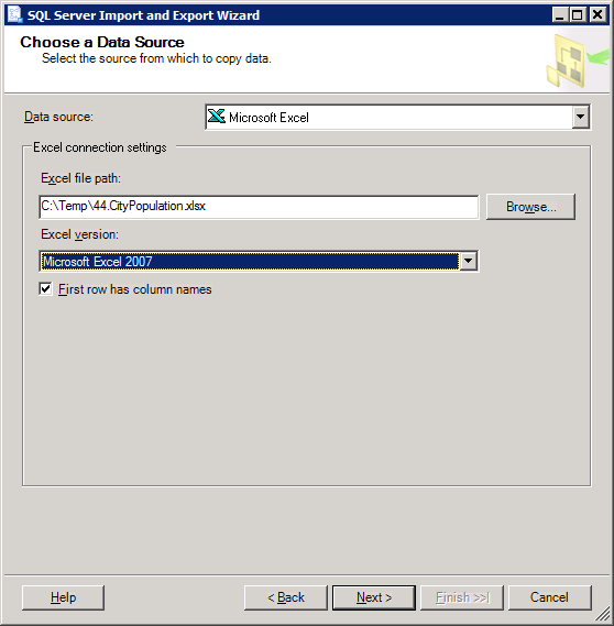
and transferred it to the SQL Server database using the Import / Export Wizard:
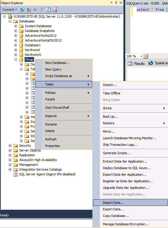
Pic.3
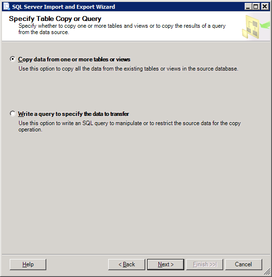
Pic.4

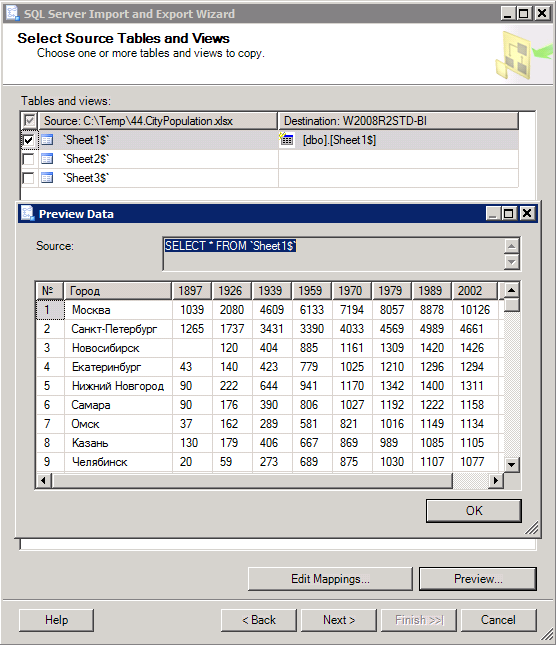
Pic.5
Pic.6
Pic.7
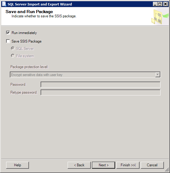
Fig.8

Fig.9
Open the structure of the imported table in SSMS (Design) and add the primary key on the field [№]:
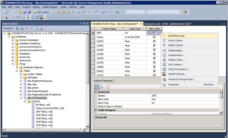
Pic.10
Previously in the SSMS settings (SSMS -> Tools -> Options) you should remove the checkbox, which by default prohibits making changes to the structure that will require re-creating the table:

Figure 11
The Import / Export Wizard transfers tables to the dbo schema. If you want to change the schema, you can do it in the same place in the table designer (F4 - Properties). In T-SQL, this corresponds to the ALTER SCHEMA ... TRANSFER command.
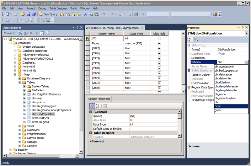
Fig.12
I think that appeared in SQL Server 2000, but the poorly known possibility is annotation of objects (Properties from the context menu -> extended properties). You can create any custom properties and set them to scalar values. In T-SQL, the stored procedures sp_addextendedproperty, sp_updateextendedproperty, sp_dropextendedproperty, and the fn_listextendedproperty function correspond to this . I will save the link from where I imported the table:
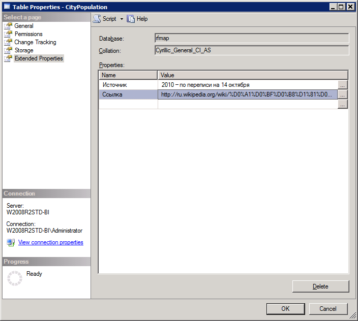
Fig.13
Now you need to add a table to the report, presenting for clarity the population by year as a trend graph in a cell opposite each city. The control is called sparkline, we passed it in this article . Initially, the CityPopulation table
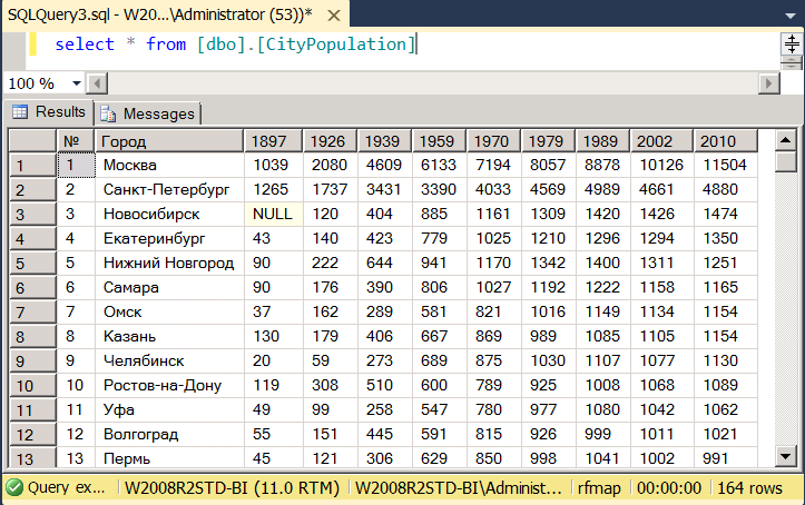
Fig.14
it is required to normalize, turning the years of 1897, 1926, ..., 2010 into columns into a separate measurement column Time running parallel to the dimension City:

Pic.15
In the report, along with the trend, I would like to display the population according to the last census of 2010. To do this, select the lines for 2010 from Fig.15 and match them with the record Fig.15 in the City column:

Figure 16
Exactly what is needed. Go to the report designer in SSDT and add a new dataset:
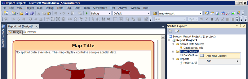
Pic.17
in which we write the data source request Fig.16. We specify the same DataSource1 as the connection on which this query will be executed, which was used to draw the map in the previous article .
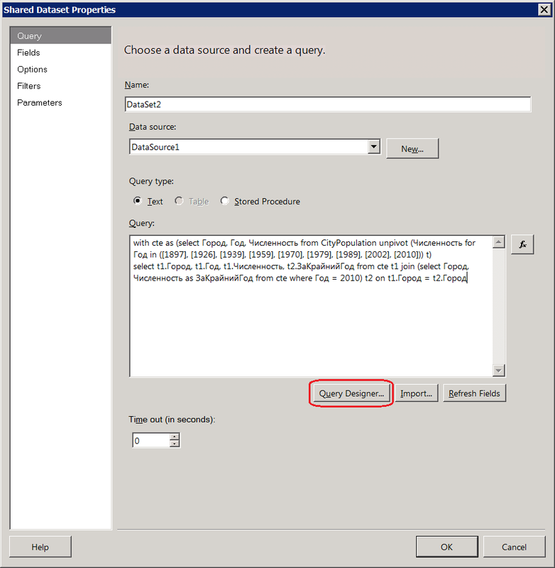
Pic.18

Figure 19
Add a Matrix control to the work surface of the report. If the panel with the fields of created datasets is not visible, it can be turned on from the top menu View -> Report Data (bottom line). Drag the City field to the 1st cell of the 2nd row of the matrix, and to the right of it we place the ZAKRIYNY field, which contains the 2010 census data. We fix the aggregate function Sum, which is substituted by default, to the aggregate function First (Expression in the properties of the cell). Or Last, or Min, or Max - not fundamental. The measure is not changed along the Time dimension. It changes only along the City dimension - Fig.16.

Pic.20
Now dataset Fig.16 is grouped by dimension City. All other measurements (Time) are collapsed. Right-click on a cell in the right column and select Insert Column -> Inside Group - Right from the context menu.

Pic.21
As the abscissa axis (Category Croups) for the trend, we add the collapsed dimension Time (Year), and on the ordinate axis we have a hidden measure of the Number, which changes along both dimensions. The Sum function, which Report Designer substitutes by default, means that if the CityPopulation table had other dimensions rolled up in the matrix, this aggregate function would be applied to them. But there are no other measurements in our case, so it’s no difference what to choose as an aggregate.
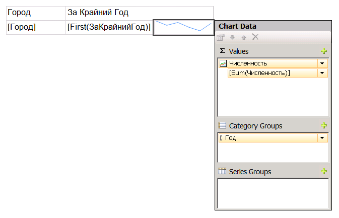
Fig.22
Spread the header cell and put the appropriate column headings.
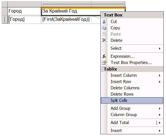
Fig.23
Adjust the font, color, alignment. Those interested can bring additional beauty. I will limit myself to removing the soft pagination in the report, so that when rendering in HTML, the entire table of cities is displayed in its entirety. To do this, in the properties panel, select in the combo box among the available controls, the Report itself, expand the InteractiveSize property and set Height = 0.

Pic.24
In order for the numbers in the middle column not to be adjacent to the graph, in the properties of the cell, it is necessary to increase Padding -> Right. But this is not the main thing. Now cities are issued in the form of a flat list, ordered alphabetically. It will probably be more beautiful to build them in accordance with the territorial hierarchy. To do this, on the CityPopulation table should have a parent-child hierarchy. Unfortunately, in the original table of Fig.1, it was absent, so it would have to be started by hand. Create a new column called ParentN and set it equal to the value of [No.] for the “parent” city. In order to save time, I will do it for cities near Moscow, since The idea is clear.
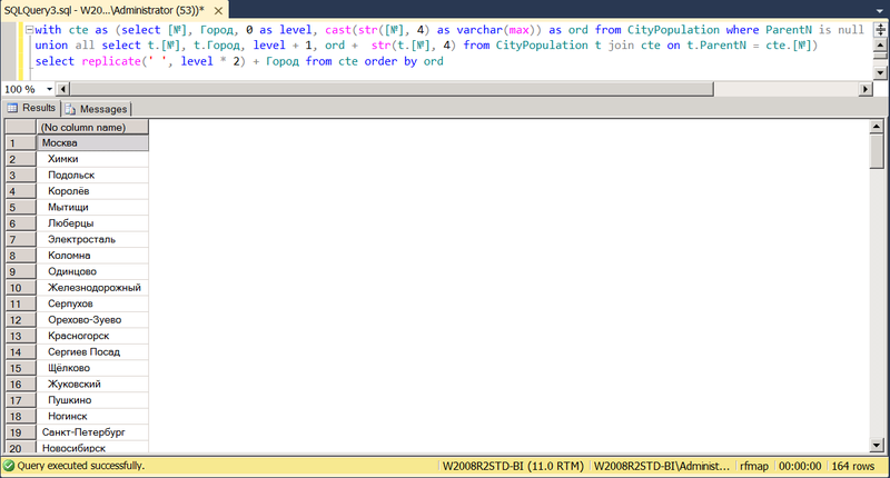
Fig.25
It's a shame that the LAG () / LEAD () functions do not work in a recursive CTE. Instead of a string, the HierarchyID could be used as the ord field, solving the task of converting the parent-child table to a hierarchy, which is called entry:
with cte as (select [No.], City, HierarchyID :: GetRoot (). GetDescendant (null, null) as hid from CityPopulation where ParentN is null
union all select t. [№], t.City, cte.hid.GetDescendant (lag (t.hid, 1) over (partition by t.ParentN order by t. [№]), null) from CityPopulation t join cte on t.ParentN = cte. [№])
select * from cte order by hid
But alas, t.hid is not perceived, so Fig.25 is in the old fashioned way. We return to the report. Change the query in DataSet2 to
To add to the ParentN field
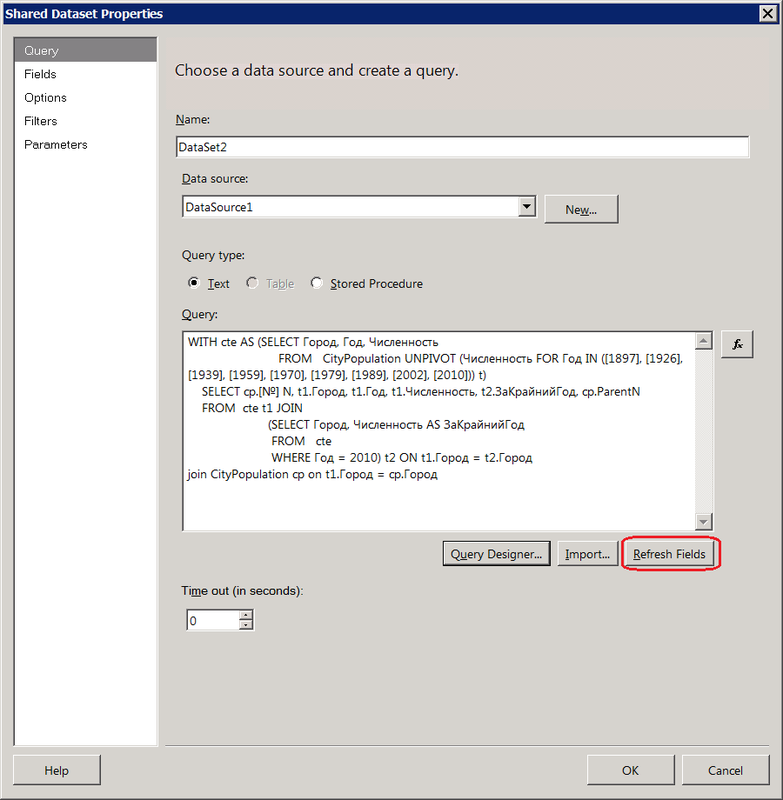
Fig.26
Click the Refresh Fields button to refresh the list of dataset fields in Report Data. The Refresh Fields button is also available if you say Edit in Report Data ...
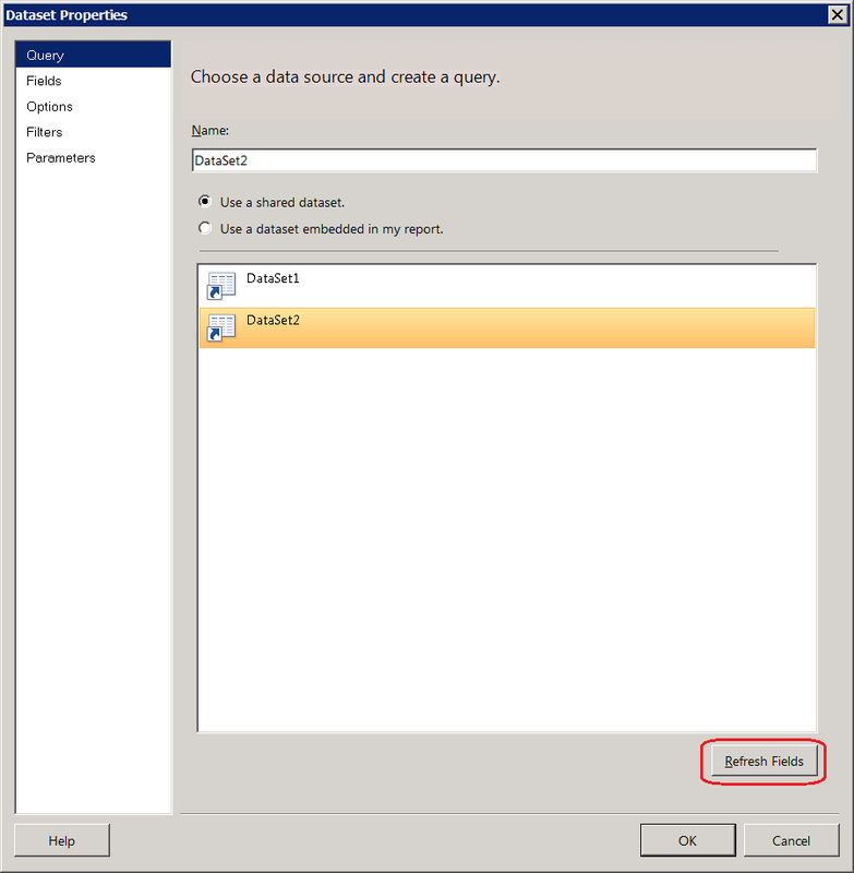
Fig.27
Open the properties of the City group:
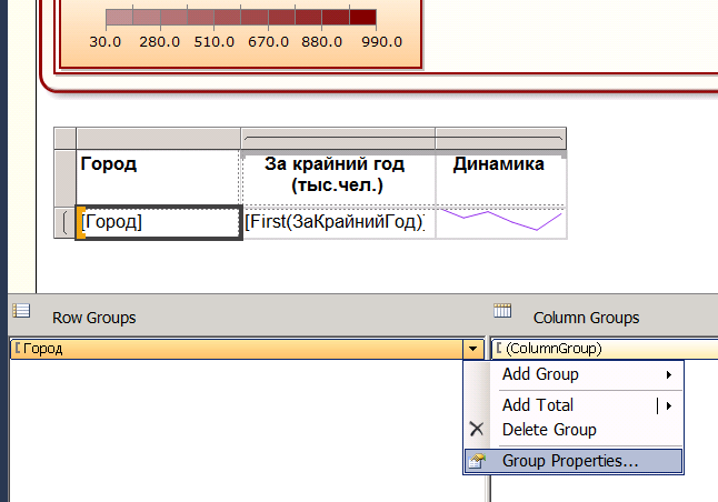
Fig.28
Change the grouping criteria from City to Field N:
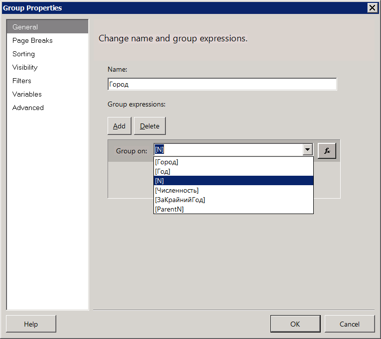
Pic.29
Stand on Advanced on the left. Select ParentN as Recursive parent, since The CityPopulation table is linked to itself in the fields No.> - ParentN. N we have just indicated in Figure 29 as, roughly speaking, the RC group. It remains to set the foreign binding key, i.e. ParentN field:

Fig.30.
Go to the Visibility tab. We say that at first everything should be in a collapsed state (Hide), and a cell named "City" (see Figure 20, Properties) should have a plus sign, by pressing which the child elements should open (Dispaly can be toggled by this report item = City):
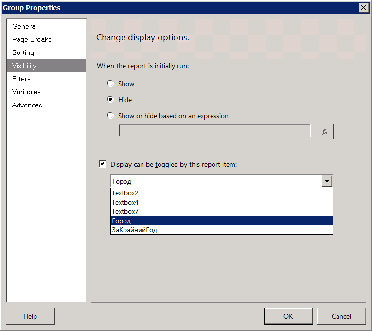
Pic.31
It remains only to emphasize the hierarchy of child elements indentation. Three things you need to remember. First, indents are adjusted using the Padding (Left) property, second, property values can include formulas (Expression), then they are dynamically evaluated on the fly, and third, the nesting level in the RS is determined by the Level (<scale>) function. Scale is the grouping in relation to which we want to get a level, i.e. in this case, the City group is bound to itself by the parent-child hierarchy. Get on the cell (Textbox) City, find Padding -> Left property in the Properties panel
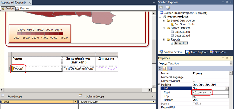
Figure 32
and set the expression for the left indent = Level ("City") * 15 & "pt":
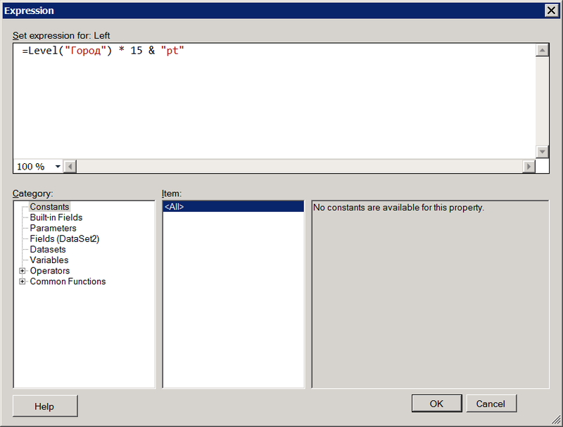
Fig.33
Run the report. Please note that now the Moscow region cities are not shown in the general list, but the + sign appears near Moscow, when clicked, it reveals its children. Empty trends for some cities mean that for the initial data of Figure 1 for them only the results of the last census were present.

Fig.34
In this example, SQL Server 2012 Developer Edition was used, because historically this has been the case. Reporting services are part of the SQL Server Express with Advanced Services edition, i.e. on the free edition is all too. in theory, should work. If anyone finds it possible to check, I will be grateful.
Pic.1
I copied the table in Excel:
Pic2
')
and transferred it to the SQL Server database using the Import / Export Wizard:
Pic.3
Pic.4
Pic.5
Pic.6
Pic.7
Fig.8
Fig.9
Open the structure of the imported table in SSMS (Design) and add the primary key on the field [№]:
Pic.10
Previously in the SSMS settings (SSMS -> Tools -> Options) you should remove the checkbox, which by default prohibits making changes to the structure that will require re-creating the table:
Figure 11
The Import / Export Wizard transfers tables to the dbo schema. If you want to change the schema, you can do it in the same place in the table designer (F4 - Properties). In T-SQL, this corresponds to the ALTER SCHEMA ... TRANSFER command.
Fig.12
I think that appeared in SQL Server 2000, but the poorly known possibility is annotation of objects (Properties from the context menu -> extended properties). You can create any custom properties and set them to scalar values. In T-SQL, the stored procedures sp_addextendedproperty, sp_updateextendedproperty, sp_dropextendedproperty, and the fn_listextendedproperty function correspond to this . I will save the link from where I imported the table:
Fig.13
Now you need to add a table to the report, presenting for clarity the population by year as a trend graph in a cell opposite each city. The control is called sparkline, we passed it in this article . Initially, the CityPopulation table
Fig.14
it is required to normalize, turning the years of 1897, 1926, ..., 2010 into columns into a separate measurement column Time running parallel to the dimension City:
select , , from CityPopulation unpivot ( for in ([1897], [1926], [1939], [1959], [1970], [1979], [1989], [2002], [2010])) t Pic.15
In the report, along with the trend, I would like to display the population according to the last census of 2010. To do this, select the lines for 2010 from Fig.15 and match them with the record Fig.15 in the City column:
with cte as (select , , from CityPopulation unpivot ( for in ([1897], [1926], [1939], [1959], [1970], [1979], [1989], [2002], [2010])) t) select t1., t1., t1., t2. from cte t1 join (select , as from cte where = 2010) t2 on t1. = t2. Figure 16
Exactly what is needed. Go to the report designer in SSDT and add a new dataset:
Pic.17
in which we write the data source request Fig.16. We specify the same DataSource1 as the connection on which this query will be executed, which was used to draw the map in the previous article .
Pic.18
Figure 19
Add a Matrix control to the work surface of the report. If the panel with the fields of created datasets is not visible, it can be turned on from the top menu View -> Report Data (bottom line). Drag the City field to the 1st cell of the 2nd row of the matrix, and to the right of it we place the ZAKRIYNY field, which contains the 2010 census data. We fix the aggregate function Sum, which is substituted by default, to the aggregate function First (Expression in the properties of the cell). Or Last, or Min, or Max - not fundamental. The measure is not changed along the Time dimension. It changes only along the City dimension - Fig.16.
Pic.20
Now dataset Fig.16 is grouped by dimension City. All other measurements (Time) are collapsed. Right-click on a cell in the right column and select Insert Column -> Inside Group - Right from the context menu.
Pic.21
As the abscissa axis (Category Croups) for the trend, we add the collapsed dimension Time (Year), and on the ordinate axis we have a hidden measure of the Number, which changes along both dimensions. The Sum function, which Report Designer substitutes by default, means that if the CityPopulation table had other dimensions rolled up in the matrix, this aggregate function would be applied to them. But there are no other measurements in our case, so it’s no difference what to choose as an aggregate.
Fig.22
Spread the header cell and put the appropriate column headings.
Fig.23
Adjust the font, color, alignment. Those interested can bring additional beauty. I will limit myself to removing the soft pagination in the report, so that when rendering in HTML, the entire table of cities is displayed in its entirety. To do this, in the properties panel, select in the combo box among the available controls, the Report itself, expand the InteractiveSize property and set Height = 0.
Pic.24
In order for the numbers in the middle column not to be adjacent to the graph, in the properties of the cell, it is necessary to increase Padding -> Right. But this is not the main thing. Now cities are issued in the form of a flat list, ordered alphabetically. It will probably be more beautiful to build them in accordance with the territorial hierarchy. To do this, on the CityPopulation table should have a parent-child hierarchy. Unfortunately, in the original table of Fig.1, it was absent, so it would have to be started by hand. Create a new column called ParentN and set it equal to the value of [No.] for the “parent” city. In order to save time, I will do it for cities near Moscow, since The idea is clear.
with cte as (select [№], , 0 as level, cast(str([№], 4) as varchar(max)) as ord from CityPopulation where ParentN is null union all select t.[№], t., level + 1, ord + str(t.[№], 4) from CityPopulation t join cte on t.ParentN = cte.[№]) select replicate(' ', level * 2) + from cte order by ord Fig.25
It's a shame that the LAG () / LEAD () functions do not work in a recursive CTE. Instead of a string, the HierarchyID could be used as the ord field, solving the task of converting the parent-child table to a hierarchy, which is called entry:
with cte as (select [No.], City, HierarchyID :: GetRoot (). GetDescendant (null, null) as hid from CityPopulation where ParentN is null
union all select t. [№], t.City, cte.hid.GetDescendant (lag (t.hid, 1) over (partition by t.ParentN order by t. [№]), null) from CityPopulation t join cte on t.ParentN = cte. [№])
select * from cte order by hid
But alas, t.hid is not perceived, so Fig.25 is in the old fashioned way. We return to the report. Change the query in DataSet2 to
WITH cte AS (SELECT , , FROM CityPopulation UNPIVOT ( FOR IN ([1897], [1926], [1939], [1959], [1970], [1979], [1989], [2002], [2010])) t) SELECT cp.[№] N, t1., t1., t1., t2., cp.ParentN FROM cte t1 JOIN (SELECT , AS FROM cte WHERE = 2010) t2 ON t1. = t2. join CityPopulation cp on t1. = cp. To add to the ParentN field
Fig.26
Click the Refresh Fields button to refresh the list of dataset fields in Report Data. The Refresh Fields button is also available if you say Edit in Report Data ...
Fig.27
Open the properties of the City group:
Fig.28
Change the grouping criteria from City to Field N:
Pic.29
Stand on Advanced on the left. Select ParentN as Recursive parent, since The CityPopulation table is linked to itself in the fields No.> - ParentN. N we have just indicated in Figure 29 as, roughly speaking, the RC group. It remains to set the foreign binding key, i.e. ParentN field:
Fig.30.
Go to the Visibility tab. We say that at first everything should be in a collapsed state (Hide), and a cell named "City" (see Figure 20, Properties) should have a plus sign, by pressing which the child elements should open (Dispaly can be toggled by this report item = City):
Pic.31
It remains only to emphasize the hierarchy of child elements indentation. Three things you need to remember. First, indents are adjusted using the Padding (Left) property, second, property values can include formulas (Expression), then they are dynamically evaluated on the fly, and third, the nesting level in the RS is determined by the Level (<scale>) function. Scale is the grouping in relation to which we want to get a level, i.e. in this case, the City group is bound to itself by the parent-child hierarchy. Get on the cell (Textbox) City, find Padding -> Left property in the Properties panel
Figure 32
and set the expression for the left indent = Level ("City") * 15 & "pt":
Fig.33
Run the report. Please note that now the Moscow region cities are not shown in the general list, but the + sign appears near Moscow, when clicked, it reveals its children. Empty trends for some cities mean that for the initial data of Figure 1 for them only the results of the last census were present.
Fig.34
In this example, SQL Server 2012 Developer Edition was used, because historically this has been the case. Reporting services are part of the SQL Server Express with Advanced Services edition, i.e. on the free edition is all too. in theory, should work. If anyone finds it possible to check, I will be grateful.
Source: https://habr.com/ru/post/146172/
All Articles