Depth of field in computer graphics

Unlike the human eye, the computer renders the entire scene in focus. Both the camera and the eye have a limited depth of field due to the final diameter of the pupil or lens aperture. To achieve greater photorealism, it is recommended to use the effect of depth of field in images obtained on a computer. In addition, the management of depth of field helps to reveal the artistic intent of the author, highlighting an important object within the meaning.

Until now, the task of imaging realistic depth of field in computer graphics has not been completely solved. There are many solutions that have pros and cons, applicable in different cases. We will consider the most popular to date.

In optics

The light, refracted in the lens, forms an image on the photosensitive element: film, matrix, retina. In order for a sufficient amount of light to enter the camera, the entrance aperture (diameter of the light beam at the entrance to the optical system) must be of sufficient size. Rays from a single point in space always converge exactly at one point behind the lens, but this point does not necessarily coincide with the selected picture plane (the sensor's half-fullness). Therefore, the images have a limited depth of field - that is, the objects will be all the more blurred, the greater the difference in distance from the object to the lens and the focal length. As a result, we will see a point located at a certain distance as a blurred spot: the scattering spot (Circle of Confusion, CoC). The blur radius is calculated according to a certain law:



Determination of the diameter of the blur (for more details, see Wikipedia ).



The methods used in renderers use the pinhole camera model (in which the input aperture → 0, and, therefore, all objects will be in focus). Simulating an aperture of finite size and, therefore, depth of field requires additional effort.

')



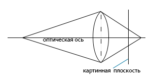
A point in the scene is projected onto the picture plane as a scattering spot.

general review

The methods for implementing depth of field can be divided into two large groups: methods of the object space (object space) and methods of the image space (image space).



Object space methods work with a 3D representation of scene objects and are thus applied during rendering. Image space methods, also known as postprocess methods, operate on raster images obtained using the standard pinhole camera model (fully in focus). To achieve the effect of depth of field, these methods blur parts of the image, taking into account the depth map (depth map). In general, object space methods are capable of producing a more physically accurate result and have fewer artifacts than image space methods, while image space methods are much faster.

Object space methods are either based on geometric optics or wave optics. Most applications use geometric optics, which is enough to achieve the vast majority of goals. However, in defocused images, diffraction and interference may play a significant role; To take them into account, it is necessary to apply the laws of wave optics.



Image space methods can be divided into those applied to generated images and applied in digital photography. Traditional post-processing techniques require a depth map, which contains information about the remoteness of the image point from the camera, but such a map is difficult to obtain for photographs. There is an interesting light field technique that allows you to blur objects that are not in focus without a depth map. The lack of technology is that it requires special equipment, but the resulting images are not limited to the complexity of the scene.

Object Space Approach Methods

Distributed ray tracing

The method directly simulates geometric optics. Instead of tracing one ray per sample (the original is a pixel, but I found it inappropriate, because the number of counted rays will vary depending on the AA settings and rarely equals one pixel), which simulates a pinhole camera, you must select several rays to get an analogue of the image obtained on the camera with the final aperture. The rays for each sample come from one point on the picture plane, but are directed to different parts of the lens. After refraction by the lens, the beam is emitted into the scene.



From the description it is clear that the image is formed, taking into account the physical laws of optics (excluding wave). Therefore, the images obtained in this way are quite realistic and are considered the “gold standard” by which you can check the post-processing methods. The disadvantage of the method is obvious: for each sample, it is necessary to calculate the number of rays sufficient to obtain a high-quality blur, respectively, the render time increases. If you want to get a shallow depth of field, you will need to increase the rendering time of hundreds or thousands of times. If you use an insufficient number of additional rays in the blurred areas, noise will appear.



The method is implemented in the mia_lens_bokeh shader:

//   struct depth_of_field { miScalar focus_plane_distance; miScalar blur_radius; miInteger number_of_samples; }; miBoolean depth_of_field ( miColor *result, miState *state, struct depth_of_field *params ) { //   miScalar focus_plane_distance = *mi_eval_scalar(&params->focus_plane_distance); miScalar blur_radius = *mi_eval_scalar(&params->blur_radius); miUint number_of_samples = *mi_eval_integer(&params->number_of_samples); miVector camera_origin, camera_direction, origin, direction, focus_point; double samples[2], focus_plane_z; int sample_number = 0; miColor sum = {0,0,0,0}, single_trace; //      miaux_to_camera_space(state, &camera_origin, &camera_direction); //    focus_plane_z = state->org.z - focus_plane_distance; miaux_z_plane_intersect(&focus_point, &camera_origin, &camera_direction, focus_plane_z); //     while (mi_sample(samples, &sample_number, state, 2, &number_of_samples)) { miaux_sample_point_within_radius(&origin, &camera_origin, samples[0], samples[1], blur_radius); mi_vector_sub(&direction, &focus_point, &origin); mi_vector_normalize(&direction); miaux_from_camera_space(state, &origin, &direction); mi_trace_eye(&single_trace, state, &origin, &direction); miaux_add_color(&sum, &single_trace); } //   miaux_divide_color(result, &sum, number_of_samples); return miTRUE; } 

The result of using the shader (the code is taken from the manual mental ray , the picture is from the same place).

Realistic camera models

In the previous method, the lens refractive index was calculated according to one law. However, this is not always the case. Lenses consist of groups of lenses with different properties:



Lens groups in the lens (picture by Pat Hanrahan).



Optical lens specifications provided by manufacturers are correctly implemented as a mathematical model. The model includes a simulation of lens groups and also provides an exit hole model (within which the renderer will emit rays for one sample). The rays entering the exit hole are calculated taking into account the optical properties of the lens groups through which they pass.



The method allows to physically correctly simulate both the depth of field and the distortion introduced by the lens.



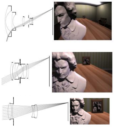
Lenses with different focal lengths: with a change in focal length and lens model, the perspective changes and there may be distortions (for example, as in the upper picture) - Pat Hanrahan image.



An example of a shader that implements a lens-fashay:

 struct fisheye { miColor outside_color; }; miBoolean fisheye (miColor *result, miState *state, struct fisheye *params ) { miVector camera_direction; miScalar center_x = state->camera->x_resolution / 2.0; miScalar center_y = state->camera->y_resolution / 2.0; miScalar radius = center_x < center_y ? center_x : center_y; miScalar distance_from_center = miaux_distance(center_x, center_y, state->raster_x, state->raster_y); if (distance_from_center < radius) { mi_vector_to_camera(state, &camera_direction, &state->dir); camera_direction.z *= miaux_fit(distance_from_center, 0, radius, 1, 0); mi_vector_normalize(&camera_direction); mi_vector_from_camera(state, &camera_direction, &camera_direction); return mi_trace_eye(result, state, &state->org, &camera_direction); } else { *result = *mi_eval_color(&params->outside_color); return miTRUE; } }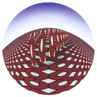 

The result of using the shader (the code is taken from the manual mental ray , the picture is from the same place).

Accumulation buffer

To achieve the effect of depth of field, you can also use an accumulation buffer. A few frames are rendered, after which, by averaging them, we get the desired image. The method is very similar to distributed ray tracing, but faster than it, since Rendering occurs using hardware. However, in the first method, we can adaptively control the number of samples and get a picture of acceptable quality, using fewer samples. The method is applicable only where it is possible to average the scene by hardware.

Waves propagation simulation

All the methods discussed above use the laws of geometric optics, ignoring diffraction and interference. If there are several point sources in the scene that emit light of a certain wavelength, you can track the propagation of light waves in space. The picture plane is located at a certain distance and to determine the value of the sample, the contribution from all the waves emitted by the sources is taken into account. Calculations can be performed in the frequency domain using the Fourier transform.

Splatting [Krivanek]

When rendering, the scene is presented not as a set of geometric primitives with textures, but as a set of points. Points are scattered according to a certain law, most often according to Gauss. To achieve higher speeds, when scattering points, the convolution operation is used, taking into account the point spread function (PSF). In the case of a Gaussian blur, the PSF parameter is the standard deviation.



The resulting points are stored in a tree and when a point is selected from a blurred area, the search is performed within a certain radius. This allows you to calculate a smaller number of samples in the out-of-focus areas of the image.



It is logical to assume that a rather rigid limitation of the method is the possibility of representing the scene in the required form.



Image obtained by the scatter method. In blurred areas, sampling density is less (picture by Jaroslav Krivanek).

Analytical visibility (Catmull)

Having a three-dimensional scene, you can analytically determine which objects are out of focus. For such objects, a smaller number of samples is taken, as a result, they look blurry. The method allows to obtain accurate images without noise, in contrast to the distributed ray tracing.

Image space methods (image space approaches)

The ideal post-processing method should have the following properties:

• Point spread function selection (PSF)
  
  The type of blur depends on the PSF, which determines which spot of scattering we will get from one point. Since this characteristic will be different in different optical systems, a good method should allow you to choose the type of PSF.
  
  
  
  Different PSF allow you to get a different nature of the blur.
• Pixel pixel control
  
  At each point in the image, the size and nature of the scattering spot is different. Typically, post-processing methods do not allow changing the nature of the blur depending on the position of the point. This is also due to the fact that often either separable filters or Fourier transforms are used in the methods, which makes such a choice difficult to implement.
  
  
  
  The first PSF image is the same; the second is changing, which more accurately simulates the Helios-44 features of some lenses.
• No intensity leakage artifacts (intensity leakage artifacts)
  
  The blurred object in the background never goes beyond the boundaries of the object in focus. However, primitive linear filters may not take this fact into account; artifacts of lack of intensity resulting from this error reduce the realism of the image.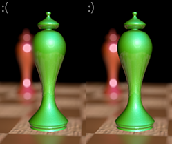
  
  
  
  The image has a green figure in focus, therefore, the blurring of an object in the background should not apply to it.
• No artifacts due to non-continuous depth (depth discontinuity artifacts)
  
  In reality, the blurring of the object in the foreground will be soft, the object will not have a visible hard contour. Often filters blur an object so that it simultaneously has both a blur and a silhouette, which is wrong. This behavior is due to the features of smoothing the depth map, with the result that the depth of the object changes in steps (and it turns out that pixels of mixed colors are on the edge of the object, as well as outside of it).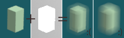
  
  
  
  The result of applying different filters. Due to the fact that the image (beauty map) is smoothed and the depth map is not, such artifacts may occur.
• Correct simulation of partial object intersection (partial occlusion)
  
  In reality, defocused objects at the front have smoothly blurred boundaries through which objects behind are visible. This effect is called a partial intersection, because the rear object is only partially blocked by the front one. We would not be able to see these visible parts of the object in the background if we looked through the pinhole camera. A geometric explanation of the effect is shown in the figure. Because post-processing methods work with images obtained on a pinhole camera; simulation of partial intersection is a difficult task: the color of invisible points must be extrapolated from the available data.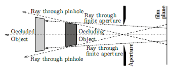
  
  
  
  Partial intersection of objects (picture Barsky).
• High performance
  
  The performance of filters applied “directly” in the image space (meaning the simplest implementation of the filter), decreases with increasing blur radius. For large radii, the process can take several minutes. Ideally, you want the filter to be applied in real time, which is not always possible.

Linear filtering [Potmesil and Chakravarty]

One of the first methods for obtaining DoF at the post-processing stage. Depending on the depth of the point (determined by the depth map), the parameters of the blur function (PSF) change. The larger the radius of the PSF, the lower the filter performance. The filter can be expressed by the formula:



where B is a blurred image, psf is the core of the filter, x and y are the coordinates in the output image, S is the original image, i and j are the coordinates in the input image.



PSF can in some sense take into account optical effects such as diffraction and interference. Disadvantages of the method: lack of intensity, non-continuous depth.

Ray distribution buffer [Shinya]

In the method it is proposed to take into account the visibility of objects, thereby we can get rid of the lack of intensity. Instead of creating a blurred image, first, for each point, a buffer is created for the distribution of the rays emanating from it. Possible coordinates are included into such a buffer, in which light can come from a point, with depth. After rendering the distribution buffers for all points, the average color value is calculated. The method works with the visibility of objects quite correctly, but requires more memory and calculations, compared to linear filtering. Note that the set of maps obtained by the RDB method is called the light field.

Layered DoF [Scofield]

The method is intended for a particular case of the location of objects: the objects must be parallel to the picture plane. Objects are divided into layers, the layers are blurred separately in the frequency domain (using the fast Fourier transform). FFT allows you to use PSF large radii without affecting performance. The method has no shortage of intensity and works very quickly, but its area of ​​application is very limited.

Intersection and discretization (occlusion and discretization) [Barsky]

The limitation imposed by the previous method is very strict. The image is divided into layers, so the depth of the image samples is rounded to the selected depth of the nearest layer. The resulting image will have discretization artifacts in the form of stripes or rigid boundaries along the lines of intersection of the layers. In this method, the problem of such artifacts is solved by using the ID of objects obtained by the method of finding boundaries (or using the ObjectId map). If one object belongs to two layers, the layers are merged. Another problem with the method is partial intersection. To blur the objects in the background, approximation by visible samples is used.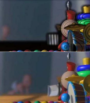



In the upper image you can see black stripes - artifacts arising from the use of layer-by-layer blur without using ObjectId (Barsky image).

Blur, taking into account the characteristics of the human eye (vision-realistic rendering) [Kolb]

The human eye is difficult to describe in the form of an analytical model consisting of several lenses - how this can be done for the lens. In this method, using a special device called a wavefront aberrometer (I did not dare to translate it), a set of PSFs corresponding to the human eye is determined. Next, blur by layers according to the PSF obtained. The method allows to obtain images visible to people with eye diseases.



An image that takes into account the peculiarities of the eye of a person with keratoconus (picture Barsky).

Importance ordering [Fearing]

The method works similarly to the renderer's antialiasing mechanism: first, an image with a low resolution is formed, after which the samples next to which the color change exceeds the threshold are processed at the next iteration and more samples of the original image are taken to obtain the pixel of the final image, and so on. Thus, the method achieves better quality in less time.

Hybrid perceptual method (perceptual hybrid method) [Mulder and van Lier]

Features of human perception of the image are such that the details in the center are more important than the details along the edges of the image. The center of the image can be blurred in a slower and more accurate way, while a fast approximation of blur is used for the periphery. For a quick blur, the Gauss pyramid is used, the blur level is selected depending on the pixel depth; the result has artifacts.

Repeated convolution (repeated convolution) [Rokita]

The method is designed for quick use in interactive applications. It works on hardware devices where it is possible to efficiently implement a convolution operation with a 3x3 pixel core. Convolution is performed several times, thereby achieving a large amount of blur. Performance drops with increasing blur radius. There is a limitation on the PSF: it must be Gaussian.

GPU depth of field [Scheueremann and Tatarchuk]

Depth of field can be considered on the GPU. One of the methods proposed Scheueremann and Tatarchuk.

Taking into account the pixel depth, according to the laws of optics, we determine the size of the scattering spot, and within the spot we select samples, which form the color of the pixel as a result. In order to optimize the memory, in areas of the image where the CoC has a large radius, pixels are taken not from the input image, but reduced in several times. To reduce the number of intensity artifacts, the depth of the pixels is also taken into account. The method has artifacts of non-continuity of depth.

Integrated matrix (summed area table) [Hensley]

As an alternative to sampling within CoC, the averaged color of the image pixel area can be found using the integral matrix (SAT). In this case, the computation speed is high and does not fall with an increase in the blur radius; moreover, there is no need to generate an image of lower resolution. Initially, the method was intended for smoothing textures, but was further adapted for depth of field, including on the GPU. The method has almost all types of artifacts.

The pyramidal method [Kraus and Strengert]

The scene is divided into layers, depending on the depth. Pixels that are close to the boundary of the layers do not belong to the closest layer, but partly to several layers: thus eliminating sampling artifacts at the boundaries of the layers. Then extrapolate the values ​​of pixels that are missing in the layers (those that are covered by objects in the foreground). After that, each layer is blurred by the pyramid method , to eliminate artifacts, the weight of the point is used. The resulting layers are mixed taking into account the transparency of the layers. The method is faster than layered methods using FFT, but imposes restrictions on the PSF used.



The image was blurred using the pyramid method (picture Magnus Strengert).

Separable Blur [Zhou]

In the same way, as in the methods of classical blur, which does not take into account depth (box blur, gaussian blur), separable PSF can be used in the calculation of the depth of field. First, the image is blurred horizontally, then vertically - as a result, we get a speed that depends not on the spot area, not on the sharpness, but on its diameter. The method is implementable on a GPU and can be applied in real time. The idea of ​​using separable functions is illustrated in the figure: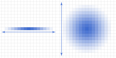



When separable blur performance depends not on the area of ​​the PSF, but on its diameter.

It is worth noting that in another work Barsky emphasizes that the correct blur, taking into account the depth, cannot be separable: when using this method, artifacts are possible in some cases.

Simulated heat diffusion [Barsky, Kosloff, Bertalmio, Kass]

Heat dissipation is a physical process in which blurring can also be observed (although it is not related to optics). If the temperature is unevenly distributed in a heat conductor, then we will observe a blur over time. Differential equations describing the effect of such a blur can be used to simulate the depth of field. Even for fairly large blur radii, the method can be applied to the GPU in real time.



The position map used instead of the depth map in this method contains information about the three dimensions of the point, and not only about the depth (Barsky image).

Generalized and semantic depth of field

So far, we have described methods that simulate depth of field as it does in nature. However, blurring may not be the same as we used to observe it. In computer graphics, we are not limited to physically feasible lens models, so the blur area can be set arbitrarily — for example, we can select several people from the crowd. The method can be implemented as a variation of the heat dissipation simulation method, using laws other than physical laws as a blurring map.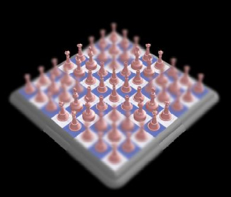



Physically incorrect blurring (picture by Kosloff and Barsky)

Light fields

The light fields were originally described as a method that describes the image of a scene from different points, regardless of the complexity of the scene. The standard way of encoding light fields is two-plane parametrization (two-plane parametrization). Two parallel planes are selected; each beam is described by a point on both planes. The result is a four-dimensional data structure. With the obtained data, you can make manipulations, such as changing the focusing plane or depth of field.



It can be said that in the cameras the light field (between the planes of the lens and the matrix) is integrated in a natural way: we do not distinguish from which point of the lens the light beam comes. However, if we take this into account, we can interactively, having the described data structure, manage the depth of field after taking the sensor readings.



In addition, we can focus on different parts of the image, applying the fast Fourier transform in four-dimensional space.



In images generated on a computer, it is easy to get the light field data by rendering the scene from different angles.



There are cameras (physical) that can record light fields. Microlenses are located in front of the sensor, separating the light coming from different directions.Thus, unlike the classical camera, the light is not summed at one point, but is distributed depending on the direction. According to the sensor, at the processing stage, you can select an object in focus and the size of the blur.





Light field: a small part of the RAW image from the Lytro sensor. We see the microlysis located in front of the matrix.

Spotted (dappled) photo

The method described above requires a lot of matrix dots to encode a single pixel, therefore, it has a low resolution. Indeed, the resolution of this camera is about 800 pixels on a larger side with an 11MPix matrix. The problem can be solved by using sensors with very high resolution (but this will lead to a rise in the cost of sensors and prohibitively large data structure size).



Spotted photography offers an alternative way to get a light field, bypassing the matrix size limit. Instead of a large number of microlens, a translucent mask is used, changing the light according to a certain law. Applying the inverse Fourier transform, you can get the original light field.

Defocus magnification

It would be nice to be able to apply the effect of depth of field in a “normal” photo, without a light field (where, unlike the render, there is no depth map). This method assumes the definition of blur and its increase (the method assumes that there is already a blur in the photo, but not enough - for example, the photo was taken on a soap box where, due to the size of the matrix, it is impossible to achieve a large blur radius). The more blur already present in the image, the more blur will be applied additionally.

Autofocus

When using depth of field in virtual reality applications and video games, as well as in photography, autofocus is necessary, that is, the problem of determining the depth, the pixels on which are in focus. In the center of the image, an area is highlighted, samples from this area are involved in determining the depth of focus. Both the weighted average depth and the intrinsic importance known to the objects depicted are taken into account (say, you can focus the “look” on one of the characters, but not on the wooden box or wall) - this is called the semantic weight of the object. It is also necessary to take into account the process of accommodation of the gaze (the focus changes smoothly in time), for this, for example, a low-pass filter is used.

Conclusion

We considered most of the most common methods used to achieve the effect of depth of field in modern computer graphics. Some of them work with 3D objects, some are post-processing methods. We also described the main characteristics that must be met by the right methods.

Currently, the problem of effectively achieving photo-realistic depth of field is still open. In addition, the problem of recreating a depth map from a photograph (determining the distance to an object) is also open.

Links

From translator

This and other works of Brian A. Barsky (University of Berkeley) can be read on his website . Wherever there are some terms and well-known names of algorithms, I left them in brackets in English, did not translate the names. If I translate somewhere incorrectly - write in a personal one, I will correct it (I studied all the terminology in English, so I could be wrong with the translation). In [square brackets] after the names of the methods are the names of those who worked on them. For the sake of clarity and interest, I supplemented the publication with examples and some pictures.