Nonlinear Dynamics and Time Series Analysis - Review of the Recurrence plots Method
Hello. In this topic, I would like to review a relatively new and quite powerful method of nonlinear dynamics - the method of Recurrence plots or recurrent analysis in the application to the analysis of time series. And, besides, it will share the code of the short program in the Matlab language, which implements everything described below.
So, let's begin. On duty, I am engaged in nonlinear dynamics, video and image processing, I would even say, a rather narrow part of nonlinear dynamics - nonlinear oscillations of rotors. As you know, the vibration signal is nothing but a time series, where the signal is the amplitude of the deviation, well, for example, the turbine rotor of the aircraft. As you know, not only the oscillations of the rotor can be represented in this form. Fluctuations of stock quotes, the activity of the Sun and many other processes are described by a simple vector of numbers, arranged in time. I will say even more, all these processes are united by one important factor - they are non-linear, and some are even chaotic, which means in practice the impossibility to predict the state in the system for an arbitrarily long period of time even knowing exactly the law of its movement in the form of differential equations. And most importantly, in most cases we cannot even write down these same equations in any form. And here comes experiment and nonlinear dynamics.
Taking readings from the sensor (downloading a file with a currency quote), we have a one-dimensional signal at the output, as a rule, of complex shape. Well even if the signal is periodic. And if not? Otherwise, we are dealing with a complex system, which, moreover, may be in the mode of nonlinear and chaotic oscillations. In this case, a complex system is a system with a large number of degrees of freedom. But we get a one-dimensional signal from the sensor. How to learn about other degrees of freedom of this system?
Before we move on to the main point, it is worth mentioning another powerful method for analyzing nonlinear dynamics, which smoothly migrated to the methods of time series analysis. This is the so-called restoration of the system trajectory from a signal from just one degree of freedom. For example, a ball is rotated in a circle on a thread, and if we are looking in the same plane at this process, we will only be able to take a signal off on one axis, for us the ball will run back and forth. And so it turned out that it is possible to completely restore the N - dimensional signal of the entire system. But not in full, but only with preservation of the topological properties of the system (more simply, its geometry). In this case, if the ball moves along a periodic trajectory, then the restored trajectory will be periodic. The method itself is based on a simple formula (in the case of a two-dimensional system):
')
Y (i) = X (t), Y1 (i) = X (t + n), where n is the time delay, and Y, Y1 is the recovered signal. This is proved in the Takens theorem. In the example, space is two-dimensional, but in reality it can be a space of an arbitrarily larger number of dimensions. The method of estimating the dimension of space is not included in the topic of this topic; I will only mention that it can be, for example, the method of false neighbors.
So, we have obtained the trajectory of the system, in which the topological properties of the real physical system are preserved, which is very important. Now we can incite a whole arsenal of pattern recognition methods on it to identify patterns. But all of them somehow have their computational shortcomings or are simply difficult to implement. And in 1987 Ekman and his colleagues developed a new method, the essence of which boils down to the following. The trajectory obtained above, which is a set of vectors of dimension N, is mapped onto a two-dimensional plane using the formulas:
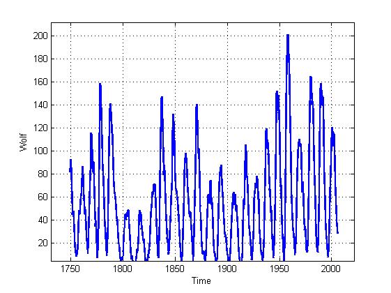
R [i, j, m, e] = O (e [i], - || S [i] - S [j] ||), where i, j are indices of a point on the plane, m is the dimension of the embedding space, O - Heaviside function || ... || - norm or distance (for example, Euclidean). The appearance of the resulting and visualized matrix will give us an idea of the dynamics of the system, initially presented in the form of a time series. We illustrate all of the above in the form of an experiment with Wolf numbers that describe the activity of the Sun (instead of this series, you can easily take quotes of currencies).
This is actually the signal itself:
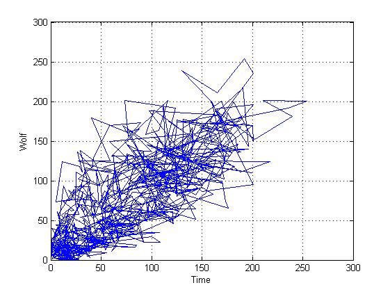
This is a reconstructed trajectory in two-dimensional space (we take two-dimensional space for simplicity, although it actually contains a greater number of dimensions, but as practice shows, this is quite enough for a qualitative assessment)
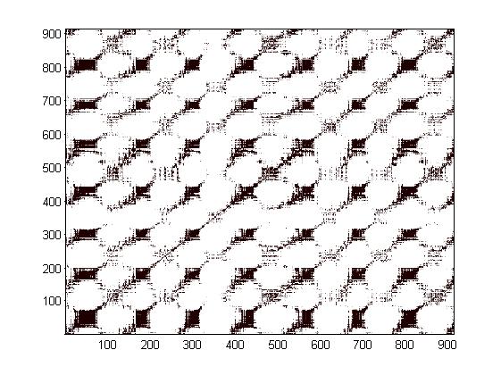
This is the so-called distance matrix (meaning only the distance from the i-th point to the j-th one). Often these diagrams have an intricate pattern that can be used (and used) in the design.

Well, here's the recurrence diagram itself. 400 pages are not enough to describe all the methods for analyzing such a diagram. In addition to qualitative analysis, this method also allows quantitative indicators, which can be successfully used in the case of using neural networks. But the most important thing is that already taking a quick look at this diagram, we can say a lot about it. Firstly, the presence of bands that are perpendicular to the main diagonal indicates the presence of chaotic or stochastic processes in the system (that would say just need more research). The presence of non-uniformly filled with black points zones indicates non-stationary processes and allows you to accurately determine the boundaries of these processes in time.
Ps. This is just an elementary example, which, naturally, does not encompass the full power of this method. In the simplest case, to automate the process, you can use the algorithms for finding shapes on the plane. Such systems may be relevant in aircraft turbine monitoring systems, as well as monitoring systems for various financial processes. I did not touch on the most interesting part of this topic - the calculation of quantitative indicators of these diagrams, which I will try to compensate in the nearest topics.
So, let's begin. On duty, I am engaged in nonlinear dynamics, video and image processing, I would even say, a rather narrow part of nonlinear dynamics - nonlinear oscillations of rotors. As you know, the vibration signal is nothing but a time series, where the signal is the amplitude of the deviation, well, for example, the turbine rotor of the aircraft. As you know, not only the oscillations of the rotor can be represented in this form. Fluctuations of stock quotes, the activity of the Sun and many other processes are described by a simple vector of numbers, arranged in time. I will say even more, all these processes are united by one important factor - they are non-linear, and some are even chaotic, which means in practice the impossibility to predict the state in the system for an arbitrarily long period of time even knowing exactly the law of its movement in the form of differential equations. And most importantly, in most cases we cannot even write down these same equations in any form. And here comes experiment and nonlinear dynamics.
Nonlinear dynamics
Taking readings from the sensor (downloading a file with a currency quote), we have a one-dimensional signal at the output, as a rule, of complex shape. Well even if the signal is periodic. And if not? Otherwise, we are dealing with a complex system, which, moreover, may be in the mode of nonlinear and chaotic oscillations. In this case, a complex system is a system with a large number of degrees of freedom. But we get a one-dimensional signal from the sensor. How to learn about other degrees of freedom of this system?
Before we move on to the main point, it is worth mentioning another powerful method for analyzing nonlinear dynamics, which smoothly migrated to the methods of time series analysis. This is the so-called restoration of the system trajectory from a signal from just one degree of freedom. For example, a ball is rotated in a circle on a thread, and if we are looking in the same plane at this process, we will only be able to take a signal off on one axis, for us the ball will run back and forth. And so it turned out that it is possible to completely restore the N - dimensional signal of the entire system. But not in full, but only with preservation of the topological properties of the system (more simply, its geometry). In this case, if the ball moves along a periodic trajectory, then the restored trajectory will be periodic. The method itself is based on a simple formula (in the case of a two-dimensional system):
')
Y (i) = X (t), Y1 (i) = X (t + n), where n is the time delay, and Y, Y1 is the recovered signal. This is proved in the Takens theorem. In the example, space is two-dimensional, but in reality it can be a space of an arbitrarily larger number of dimensions. The method of estimating the dimension of space is not included in the topic of this topic; I will only mention that it can be, for example, the method of false neighbors.
Recurrence plots method
So, we have obtained the trajectory of the system, in which the topological properties of the real physical system are preserved, which is very important. Now we can incite a whole arsenal of pattern recognition methods on it to identify patterns. But all of them somehow have their computational shortcomings or are simply difficult to implement. And in 1987 Ekman and his colleagues developed a new method, the essence of which boils down to the following. The trajectory obtained above, which is a set of vectors of dimension N, is mapped onto a two-dimensional plane using the formulas:
R [i, j, m, e] = O (e [i], - || S [i] - S [j] ||), where i, j are indices of a point on the plane, m is the dimension of the embedding space, O - Heaviside function || ... || - norm or distance (for example, Euclidean). The appearance of the resulting and visualized matrix will give us an idea of the dynamics of the system, initially presented in the form of a time series. We illustrate all of the above in the form of an experiment with Wolf numbers that describe the activity of the Sun (instead of this series, you can easily take quotes of currencies).
results
This is actually the signal itself:
This is a reconstructed trajectory in two-dimensional space (we take two-dimensional space for simplicity, although it actually contains a greater number of dimensions, but as practice shows, this is quite enough for a qualitative assessment)
This is the so-called distance matrix (meaning only the distance from the i-th point to the j-th one). Often these diagrams have an intricate pattern that can be used (and used) in the design.
Well, here's the recurrence diagram itself. 400 pages are not enough to describe all the methods for analyzing such a diagram. In addition to qualitative analysis, this method also allows quantitative indicators, which can be successfully used in the case of using neural networks. But the most important thing is that already taking a quick look at this diagram, we can say a lot about it. Firstly, the presence of bands that are perpendicular to the main diagonal indicates the presence of chaotic or stochastic processes in the system (that would say just need more research). The presence of non-uniformly filled with black points zones indicates non-stationary processes and allows you to accurately determine the boundaries of these processes in time.
Matlab Code
clear; clc;
%
[X1,X2,X3,X4]=textread('data.txt','%f %f %f %f');
plot(X2,X4);grid;hold; ; ylabel('Wolf');xlabel('Time');
N = length(X1);
M = round(0.3*N);
M1 = N - M;
m = 2; %
t = 10; %
%
X(1,1) = 0;
X(1,2) = 0
j = 1;
%
for i=M1:(N - t)
X(j,1) = X3(i);
X(j,2) = X3(i + t);
j = j + 1;
end
figure;
plot(X(:,1),X(:,2));grid;hold; ; ylabel('Wolf');xlabel('Time');
N1 = length(X(:,1))
D1(1,1) = 0;
D2(1,1) = 0;
e = 30;
% RP -
for i = 1:N1
for j = 1:N1
D1(i,j)=sqrt((X(i,1)-X(j,1))^2+(X(i,2)-X(j,2))^2);
if D1(i,j) < e
D2(i,j) = 0;
else
D2(i,j) = 1;
end;
end;
end;
figure;
pcolor(D2) ;
shading interp;
colormap(pink);
figure;
pcolor(D1) ;
shading interp;
colormap(pink);
hold on
Ps. This is just an elementary example, which, naturally, does not encompass the full power of this method. In the simplest case, to automate the process, you can use the algorithms for finding shapes on the plane. Such systems may be relevant in aircraft turbine monitoring systems, as well as monitoring systems for various financial processes. I did not touch on the most interesting part of this topic - the calculation of quantitative indicators of these diagrams, which I will try to compensate in the nearest topics.
Literature
- J.-P. Ecmann N S. Oliffson Kamphorst and D. Ruelle, Recurrence Plots of Dynamical Systems
- www.recurrence-plot.tk
- en.wikipedia.org/wiki/Recurrence_plot
Source: https://habr.com/ru/post/145805/
All Articles