Kopules - what it is and what they are
This resource often speaks about working with random variables - well, a lot of where they are needed. Sometimes it happens that you need to determine the dependence of two random variables on each other. Here you will exclaim - "Pfff, so we are in school - correlation." Here I want to upset you - Pearson's correlation is just one of many ways to show the dependence of two random variables. In addition, it is linear. That is, if the relationship between X and Y is not linear, but, say, quadratic, that is, X = Y ^ 2, then the Pearson correlation will show the absence of dependence. But we know that it is not. If you have not thought about this before, now you should have ideas - “How is that?”, “And what can we do?”, “Aaaa, we will all die!” I will try to give answers to all these difficult questions under the cut .
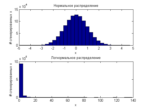
To begin, let me remind you that the cumulative distribution functions can be defined on any set of values, but they themselves have values from 0 to 1. That is, they convert values from a given set to a strictly defined range from 0 to 1. You can imagine that they “archive” . For example, the normal function "archives" the range from minus infinity to plus infinity to this most notorious (0.1). Lognormal distribution "archives" the range only from 0 to infinity. And so on.
Now imagine the process of "unarchiving". It is made by inverse distribution functions. They are also called quantile functions. You already understood the point - these functions transform the range (0,1) into the range of values specified by this function. All this, of course, with a bunch of restrictions, but for the "visual presentation", such a comparison is quite suitable.
What is interesting is if we take 10 ^ 6 random variables generated according to the same principle (for example, the standard normal distribution) and another 10 ^ 6 according to the lognormal distribution law:
and then “archive” them, then the two million values obtained will be evenly distributed from 0 to 1.
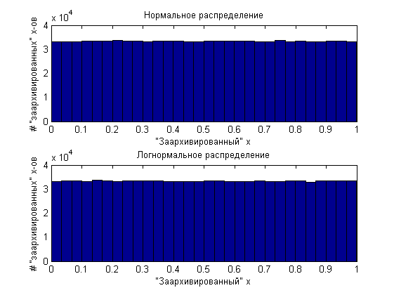
That is, in fact, any distribution can be generated from uniformly distributed values and the inverse distribution function. There would be such a function. On this educational program we will finish.
')
Now introduce you to the copula. The formula definition is:

where u is the “archived” value (u = F (x), F is the marginal distribution function). We can also write that

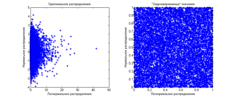
That is, it is a joint distribution function of several “archived” values. You can say - "uh ... we just showed that the" archived "values are equally distributed for all distribution functions." This is true for individual quantities, we work with several at once. Suppose we have two values — one is normally distributed, the other is lognormal. For starters, they will be independent of each other. Marginal (when we consider values separately) distributions we have already shown above. Now I will show how their joint distribution looks like:
As you can see, the “archived” values are evenly distributed over a square of 1 by 1. Now we will generate the same values, but let's say that there is a correlation between them equal to 0.8. The result is shown in the following graph.

As you can see, now the distribution of “archived” values is uneven - it is more concentrated diagonally. Here the limited use of correlation, as a measure of the dependence of quantities, is manifested. By operating only with it, you can distribute the “archived” values only closer or farther from the diagonal. The diagonal will be either 45 degrees if the correlation is positive, or 135 degrees if the correlation is negative. What if you want to show another dependency pattern? This is where the copulas come to your rescue. From the formula definition of a copula it can be seen that it shows the distribution function on this square 1 for 1, if there are two quantities. If there are more than two, then the copula will show the distribution in the n-dimensional cube 1 on 1 on 1 ... by 1. Using different copulas, you can show any distributions of the “archived” values. Another important advantage of copulas is their independence from marginal distributions. That is, you do not care what marginal distributions have values - you work directly with the dependencies expressed through the dependencies of the “archived” values.
Since a copula is still a function of probability, and not a distribution of quantities as such, it is graphically shown as a surface for which each point is equal to the joint probability of two quantities. In other words, it is a plot of joint distribution density. For clarity, I will give an example of several copulas:
To begin, let us show the Gaussian copula density distribution function itself (gaussian copula) as well as its graphic display:

Where Is the normal distribution function, and
  - the inverse function of the i-th marginal distribution, that is, the distribution of a specific value per se.
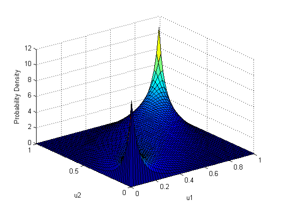
As you can see, it is very similar to the distribution of “archived” random variables in the last example. There is nothing strange in this, since the last example used just a Gaussian copula with the same correlation parameter of 0.8, with normal and lognormal marginal distribution functions.
Next I would like to show Student Copula (Student Copula):

Where t is the Student’s distribution function with a given covariance matrix and a given number of degrees of freedom
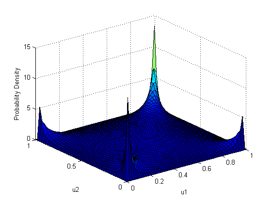
It can be seen that, unlike the Gaussian copula, the Student’s copula has a greater value at the extreme values (1-1 and 0-0), which means thicker distribution tails. Even more noticeable are the high values in the corners 0-1 and 1-0, which means a pronounced inverse relationship at the ends of the ranges of definitions of marginal functions. It should be noted that this graph was constructed for a positive correlation between the values. In the case of zero correlation, in contrast to the Gaussian copula, where in this case there would be a uniform distribution over all the squares, the Student’s tug has the same weights for all angles. This means that if one value takes a "tail" value, the other will also take a "tail" value, but with equal probability, right or left. For ease of reading the graph of the density of the copula, you can mentally make a slice perpendicular to one of the axes. The resulting graph will be a graph of the probability density of the loss of one "archived" value while fixing another.
I would also like to show Clayton copula (Clayton copula), which determines the degree of coherence of the two quantities only by the alpha parameter, which must be strictly greater than 1.


Here, the main weight lies at 0–0, that is, the values will most likely take values from the left tail of the margin functions.
In general, copulas make it possible to show any dependence of several quantities on each other, expanding the range of modeling. For further reference, I cite a small list of references.
Copula in Matlab
Understanding relationships using copulas - Edward Frees, Emiliano Valdez
Coping with copulas - Thorsten Schmidt
To begin, let me remind you that the cumulative distribution functions can be defined on any set of values, but they themselves have values from 0 to 1. That is, they convert values from a given set to a strictly defined range from 0 to 1. You can imagine that they “archive” . For example, the normal function "archives" the range from minus infinity to plus infinity to this most notorious (0.1). Lognormal distribution "archives" the range only from 0 to infinity. And so on.
Now imagine the process of "unarchiving". It is made by inverse distribution functions. They are also called quantile functions. You already understood the point - these functions transform the range (0,1) into the range of values specified by this function. All this, of course, with a bunch of restrictions, but for the "visual presentation", such a comparison is quite suitable.
What is interesting is if we take 10 ^ 6 random variables generated according to the same principle (for example, the standard normal distribution) and another 10 ^ 6 according to the lognormal distribution law:
and then “archive” them, then the two million values obtained will be evenly distributed from 0 to 1.
That is, in fact, any distribution can be generated from uniformly distributed values and the inverse distribution function. There would be such a function. On this educational program we will finish.
')
Now introduce you to the copula. The formula definition is:
where u is the “archived” value (u = F (x), F is the marginal distribution function). We can also write that
That is, it is a joint distribution function of several “archived” values. You can say - "uh ... we just showed that the" archived "values are equally distributed for all distribution functions." This is true for individual quantities, we work with several at once. Suppose we have two values — one is normally distributed, the other is lognormal. For starters, they will be independent of each other. Marginal (when we consider values separately) distributions we have already shown above. Now I will show how their joint distribution looks like:
As you can see, the “archived” values are evenly distributed over a square of 1 by 1. Now we will generate the same values, but let's say that there is a correlation between them equal to 0.8. The result is shown in the following graph.
As you can see, now the distribution of “archived” values is uneven - it is more concentrated diagonally. Here the limited use of correlation, as a measure of the dependence of quantities, is manifested. By operating only with it, you can distribute the “archived” values only closer or farther from the diagonal. The diagonal will be either 45 degrees if the correlation is positive, or 135 degrees if the correlation is negative. What if you want to show another dependency pattern? This is where the copulas come to your rescue. From the formula definition of a copula it can be seen that it shows the distribution function on this square 1 for 1, if there are two quantities. If there are more than two, then the copula will show the distribution in the n-dimensional cube 1 on 1 on 1 ... by 1. Using different copulas, you can show any distributions of the “archived” values. Another important advantage of copulas is their independence from marginal distributions. That is, you do not care what marginal distributions have values - you work directly with the dependencies expressed through the dependencies of the “archived” values.
Since a copula is still a function of probability, and not a distribution of quantities as such, it is graphically shown as a surface for which each point is equal to the joint probability of two quantities. In other words, it is a plot of joint distribution density. For clarity, I will give an example of several copulas:
To begin, let us show the Gaussian copula density distribution function itself (gaussian copula) as well as its graphic display:
Where
Is the normal distribution function, and - the inverse function of the i-th marginal distribution, that is, the distribution of a specific value per se.As you can see, it is very similar to the distribution of “archived” random variables in the last example. There is nothing strange in this, since the last example used just a Gaussian copula with the same correlation parameter of 0.8, with normal and lognormal marginal distribution functions.
Next I would like to show Student Copula (Student Copula):
Where t is the Student’s distribution function with a given covariance matrix and a given number of degrees of freedom
It can be seen that, unlike the Gaussian copula, the Student’s copula has a greater value at the extreme values (1-1 and 0-0), which means thicker distribution tails. Even more noticeable are the high values in the corners 0-1 and 1-0, which means a pronounced inverse relationship at the ends of the ranges of definitions of marginal functions. It should be noted that this graph was constructed for a positive correlation between the values. In the case of zero correlation, in contrast to the Gaussian copula, where in this case there would be a uniform distribution over all the squares, the Student’s tug has the same weights for all angles. This means that if one value takes a "tail" value, the other will also take a "tail" value, but with equal probability, right or left. For ease of reading the graph of the density of the copula, you can mentally make a slice perpendicular to one of the axes. The resulting graph will be a graph of the probability density of the loss of one "archived" value while fixing another.
I would also like to show Clayton copula (Clayton copula), which determines the degree of coherence of the two quantities only by the alpha parameter, which must be strictly greater than 1.
Here, the main weight lies at 0–0, that is, the values will most likely take values from the left tail of the margin functions.
In general, copulas make it possible to show any dependence of several quantities on each other, expanding the range of modeling. For further reference, I cite a small list of references.
Copula in Matlab
Understanding relationships using copulas - Edward Frees, Emiliano Valdez
Coping with copulas - Thorsten Schmidt
Source: https://habr.com/ru/post/145751/
All Articles