or how mismatched lines spoil your signal

On the Dangerous Prototypes forum, I once took part in one discussion on SPI bus problems, which stopped working normally, starting at a certain length. My experience suggested two things to me: 1) check the power source, 2) check the line for reflections. Then I realized that this should be a common problem for all radio amateurs. Data lines are a complex topic, and it is time to remove the cover of mystery from this electronic magic.

Introduction

It's one thing to collect something interesting from the LEDs, the controller, and several logic packages. And it is quite another to connect your creation with the outside world with cables and try to transmit various low and high frequency signals through them. The laws of physics are relentless, and developing good data lines is not a trivial task in and of itself.

My first practical acquaintance with long lines took place about 20 years ago when I tried to transmit a 8 MHz CGA digital video signal over a 15-25 m cable. As you can imagine, my first attempt was not successful. I learned about long lines almost ten years earlier, but I never used this knowledge in practice. Thus, I had to specifically delve into the study and understand the problem.

The theory of long lines is clear enough, but it can frighten those who do not understand analog electronics. Just know that you can’t avoid meeting long lines. You will surely come across them at some stage of your activity, and you will have to solve problems that arise.
')
Fortunately, there are several relatively simple things you can do to save yourself from defeat. The problems caused by long lines can be easily seen (with the help of an oscilloscope. - Approx. Transl. ) , And then I clearly, with a lot of pictures, try to show you what happens to the signals of different frequencies in different transmission lines.

Here, for example, the oscillogram of the signal at the cable output:


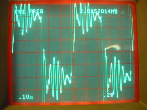
Figure 1. The signal at the line output without taking special measures.

Our beautiful signal is now disfigured.

What is the long line?

Any connection can be considered as a long line. However, characteristic effects are not always observed. That is why there are several definitions, which line is considered to be long. It depends on what area you work in. You should understand that the signal takes time to travel from one to the other end of the cable. That's the whole point.

In the copper wire, the signal is transmitted at a speed of about 2/3 of the speed of light (about 2 · 10 ⁸ m / s). This means that every 20 cm of cable will give 1 ns delay. These numbers allow you to estimate how much you can lengthen the line before trouble begins.

When you transmit a variable signal through a cable, at a certain frequency a situation will arise that the input voltage has already changed phase, and the signal has not yet reached the output. In fact, the problems will begin long before the whole signal period in the cable begins to fit.

The following long line definitions are commonly used:

• a line transmitting signals of such high frequencies that the wavelength must be taken into account (Wikipedia);
• a line transmitting such a signal that a half-wave or more fits along the length of the line;
• line, the length of which fits a significant part of the wavelength.

This theory ends. Let us show in practice what is happening, trying to use the minimum set of devices and parts.

Measuring installation

The OSAA site kindly provided all the necessary materials. Here is what I used:

• 20 meters of unshielded twisted pair of the 5th category;
• another half a meter of the same twisted pair (to show that with short cables is not so simple);
• signal generator;
• two oscillographs with a 100 MHz bandwidth;
• dual power supply;
• breadboard;
• two RJ-45 connectors.

The following scheme was assembled:


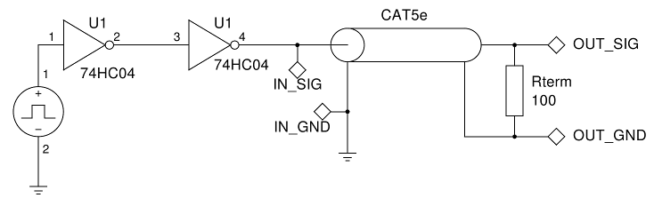
Figure 2. Line power supply circuit with low current output

The circuit is simply a 74HC04 inverter loaded on a cable. The power supply voltage is 5 V. The oscilloscope No. 1 is connected to the IN_SIG / IN_GND points, and the oscilloscope No. 2 is connected to the OUT_SIG / OUT_GND. It is important to note that the oscilloscopes are not connected to a common ground . Connecting their common wires together will mean shorting the line. An Rterm resistor, called a terminator , can be connected or disconnected. When Rterm is disabled, the line is called open or non-terminated .

The second circuit is a cascade with a high-current output. Several 74HC04 inverters are connected in parallel, each equipped with a current-leveling resistor of 10 ohms. This should provide a current of up to several hundred milliamps. This scheme simulates the power line from special driver chips.


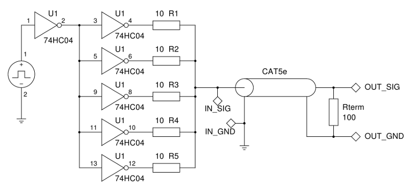
Figure 3. Line power supply circuit with high current output

Note: diagrams are for illustration purposes only. In real life, additional requirements may be imposed on circuits, which are described later in this article.

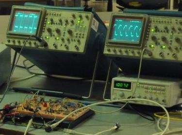
The assembled installation looks like this:


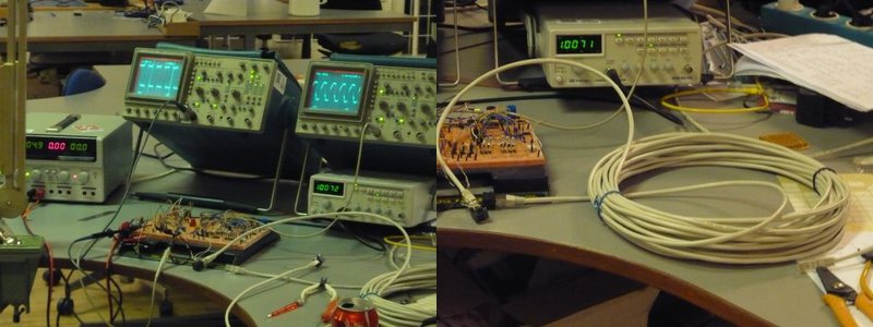
Figure 4. Measuring installation


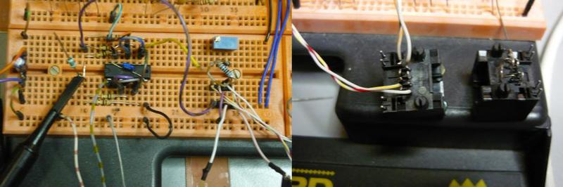
Figure 5. Development board and connectors

The RJ-45 connectors, as shown in Figure 5, were connected in a special way. The cable consists of four twisted pairs, and thus we can explore a line of greater length if we connect different pairs of cables in series. Jumpers on the connectors connect the pairs between each other, that is, the effective cable length is quadrupled. From the 20-meter cable turns 80-meter transmission line.

Since most of the equipment was donated, it was a problem to find two devices of the same brand, model and version. The cables of the oscilloscope probes used for measurements differed from each other by 30 cm in length. As mentioned above, this introduces a delay in signal propagation through the cable. So, if you connect one oscilloscope with different probes to the same signal source, you will notice a slight difference in the results:


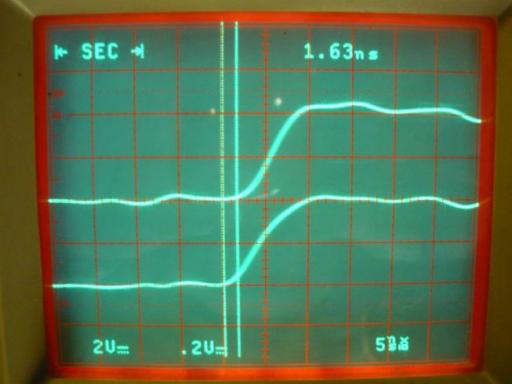
Figure 6. The propagation delay caused by a 30 centimeter difference in the length of the wires

The measured delay was 1.6 ns. This may seem a bit, but when trying to match two signals that are close to each other in time, you need to take into account the length of the cable.

Note: the oscilloscope shows the resolution on the Y axis of 2 V / div and 0.2 V / div for different channels. Both probes have a 1:10 divider, but only one of them has a special label that allows the oscilloscope to recognize the type of probe and correctly display the vertical resolution. In fact, the resolutions of both channels are the same.

The first measurement shows the delay introduced by 80 meters of cable. Here, the input and output signals are fed to the same oscilloscope. This is the only measurement where it is permissible to use a single oscilloscope, since the common wire of the line is short-circuited, as mentioned above. Nevertheless, it is possible to show the signal delay in a simple way.


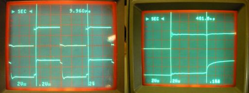
Figure 7. The delay of signal propagation in the 80-meter cable (the upper channel is the input, the lower one is the output)

The enlarged image (Fig. 7, right) shows a delay of 402 ns, which corresponds to a line length of 2 · 10 ⁸ m / s · 402 · 10 ^-9 s = 80.4 m. Very close to what was expected, so we can assume The result is acceptable.

Long line measurements

When the installation is ready, you can start the real measurements. What happens if you apply a 100 kHz square wave to an 80-meter cable? Answer: depends on how well you agreed on the line.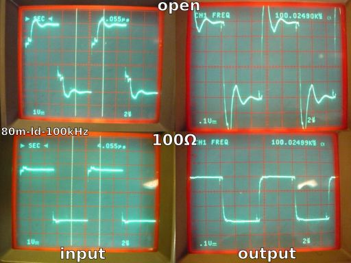


Figure 8. Cable 80 m, signal 100 kHz, low-current line power.
Upper row: non-terminated line, on the left - the entrance, on the right - the exit.
Bottom row: the terminated line, on the left - the entrance, on the right - the exit

What's going on here? Non-terminated cable gives a bunch of garbage, both at the output and at the entrance . When the resistance of 100 ohms is connected to the cable, everything looks good. The answer lies in the properties of the long line. When you bring a signal to the cable, you transmit energy to the cable. This energy spreads through it until it reaches the end, which takes time , and then it must come out of the cable. However, if there is high resistance at the end of the cable, energy cannot escape from the cable and is reflected back to the input. (At too low resistance (short circuit) at the end of the line, the energy is also reflected, only the phase of the reflected signal will be different. - Appro. Transl. )

Some of you may have seen a rope experiment in a physics lesson in school. You take the rope, fix it with one end against the wall, stretch it and swing the free end. You can see that the impulse sent along the rope reaches the wall, is reflected and runs back. The long line does the same thing, only with electricity.

Any long line has a parameter called line impedance . No matter how long the cable is, it has the same characteristic impedance. To pick up the energy that is transmitted through the cable, the end resistance must be equal to the characteristic impedance of the line. In the case of a twisted pair is 100 ± 15 Ohms. For any cable, the characteristic impedance is either known or can be measured.

The reason for which the resistance of the terminator should be equal to the characteristic impedance of the line is based on the maximum power theorem (Jacobi theorem) . To transmit the maximum power, the internal resistances of the source and the receiver of the energy must be the same. Any terminator whose resistance is not equal to the line impedance allows part of the energy to be reflected back into the cable from it.

You can measure the characteristic impedance of any cable by changing the terminator's resistance (take a variable resistor) until the reflection disappears. For the applied cable, this technique gave the result of 114 ohms. According to the cable specification, this is within the normal range.

If you are thinking now: “Why can't I use a cable with infinite characteristic impedance?”, I have to disappoint you, because the attenuation of the signal in the cable is due to its characteristic impedance. The higher the cable impedance becomes, the harder it is to transmit a signal through it. Energy is absorbed by the cable, but nothing comes to the output. Conversely, an impedance equal to zero will give a cable without attenuation (lossless), the output will have to create a short circuit, which means that the output voltage will be zero.

Note trans .: The above is not quite right. Attenuation coefficient does not depend on wave resistance. Both of these parameters depend on the geometric dimensions of the line and on the properties of the materials from which it is made. By applying ideal conductors and insulators, it is possible to create a line without attenuation with any given characteristic impedance. On the other hand, when using real materials, a higher impedance cable will have greater attenuation, ceteris paribus. Another reason why high-resistance lines are not used is the difficulty of matching them with the signal source.

As can be seen from Figure 8, even a not very high-frequency 100 kHz signal is littered. Let's raise the frequency to 1 MHz and see what happens:


Figure 9. Cable 80 m, 1 MHz signal, low-current line power.
Upper row: non-terminated line, on the left - the entrance, on the right - the exit.
Bottom row: the terminated line, on the left - the entrance, on the right - the exit

At high frequencies, there is a new effect. Signal fronts are no longer steep, but of exponential form, even with proper matching. A driver on one logical element cannot transfer energy to the cable fast enough. Each cable has its own capacity, which is usually specified per meter or kilometer length. According to the specification, the cable of the 5th category has a capacity of 52 pF / m. With a length of 80 m, the capacity is 4.16 nF.

Looking carefully at Figure 9 (bottom right), one can see that the front beginning is steep and almost linear. The voltage rise on the first 1.8 V is almost linear in 40 ns. During this short time, the output buffer of the inverter outputs a current I = (U · C) / T = (4.16 nF · 1.8 V) / 40 ns = 187 mA (!)

Then follows the exponential part of the curve. Its shape depends on the driver settings, as well as on the resistance, capacitance and inductance of the cable. The exact calculation of this curve is a complex integral calculation, beyond the scope of this article.

A source is required that can deliver a much higher current in order to overcome the cable capacitance and again make the waveform look like something “normal”. So, once again we will carry out measurements at low and high frequencies for a high-current circuit (Fig. 3):


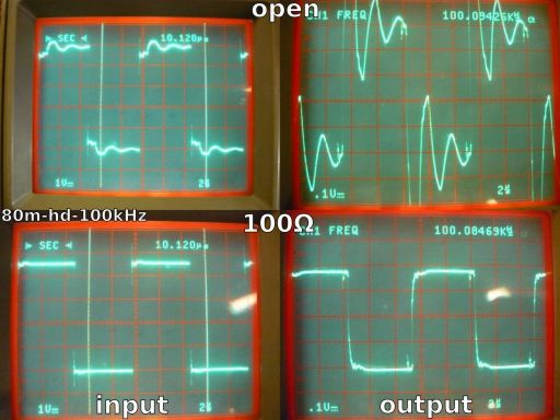
Figure 10. 80 m cable, 100 kHz signal, high current line power.
Upper row: non-terminated line, on the left - the entrance, on the right - the exit.
Bottom row: the terminated line, on the left - the entrance, on the right - the exit

Using a powerful scheme has two implications. First, the energy pumped into the cable is much higher. Thus, a large amount of energy will be reflected in the mismatched cable (Fig. 10, upper right). This may cause damage to the equipment, since the output voltage is much higher than 5 V.

Secondly, with the correct alignment, the edges of the signal are again steep and clear. You can also see that the voltage is at an acceptable level for digital circuits of 3.8 V (Fig. 10, bottom right).

The output voltage of the installation is limited by the resistances of the cable and the DC load. The entire cable has a DC resistance of 2 · 80 m · 0.188 Ω / m = 30 Ω. Please note that cable resistance consists of the resistance of two wires of 80 m each. The cable together with the 100 ohm terminator form a voltage divider. The maximum voltage at the output of the divider is 5 V · 100 Ω / (100 Ω + 30 Ω) = 3.85 V. The measured value is very close to theoretical. Not bad for a "knee" assembly.

Cable resistance is one of the reasons why you cannot close IN_GND and OUT_GND pins between each other (see fig. 2 and 3). The return path from OUT_GND to IN_GND has a resistance of 15 Ohms, and the voltage drops to about 0.58 V.

If you close the ground, you eliminate part of the cable from work and actually create an earth loop . Part of the reverse current will flow through the cable, and part through the point of the circuit. The problem, however, is that the length and properties of the cable and the shorted section are not the same, and the difference in signal propagation along these two paths will play a significant role. That is, the Bad Stuff ™ will happen if you close the land between them.

Consider a 1 MHz signal with a high-current driver:


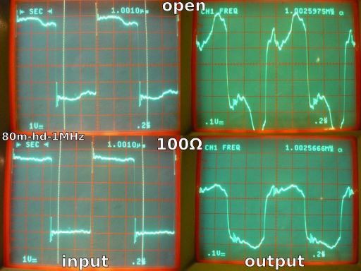
Figure 11. 80 m cable, 1 MHz signal, high current line power.
Upper row: non-terminated line, on the left - the entrance, on the right - the exit.
Bottom row: the terminated line, on the left - the entrance, on the right - the exit

As can be seen from Figure 11, the signal at the output of a cable with high-current power has an acceptable shape if it is matched. The estimated peak current is (4.16 nF · 2.5 V) / 20 ns = 520 mA (!). You can imagine what a huge load falls on the driver during signal transmission.

The high impulse current required to transmit a signal through a cable is the reason for which specialized chips are used - line and bus drivers. These chips are designed to provide very high currents for a short time without burning out. You should also make sure that you have supplied these circuits with proper decoupling capacitors .

Short cable, big problems

So far, we have only considered long cables. However, the feature of the long line is that its characteristic impedance does not depend on the length. Translating into human language: even using a short cable, you can not relax.

Remove the 20-meter cable, replace it with a half-meter piece and measure the signal propagation delay:


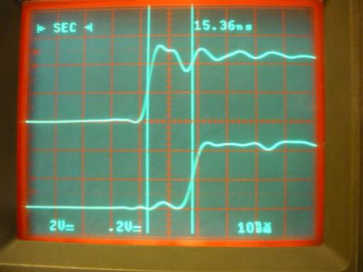
Figure 12. Propagation delay in the 2.3-meter line (top - input, bottom - output)

The expected delay in a 4 × 0.5 m cable should be about 10 ns, but measurements show a value far from the calculated one. There are several explanations for this:

• test leads have different lengths: 1.6 ns errors;
• the connectors are connected to the board with a 15 cm wire: twice 0.75 ns;
• The purple wire from the driver to the cable (Fig. 5, left) has a length of 10 cm: another 0.5 ns errors;
• The signal speed in the cable is less than 2/3 of the speed of light. In accordance with the cable specification, about 0.64 · s: 4% error;
• Twisted pair has a greater electrical length than the cable itself, due to the fact that the conductors go in a spiral: the quantitative difference is unknown.

Summing up these errors, except for the last one, and taking the cable length along with the leads (2.3 m), we obtain a calculated delay of 12.7 ns, which corresponds to a line length of 2.4 m. Already much closer to reality.

What happens if a 100 kHz signal is transmitted over this not-very-long line?


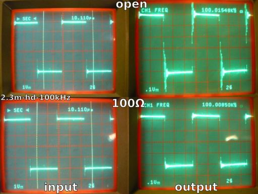
Figure 13. Cable 2.3 m, 100 kHz signal, high current line power.
Upper row: non-terminated line, on the left - the entrance, on the right - the exit.
Bottom row: the terminated line, on the left - the entrance, on the right - the exit

Answer: if you do not agree on the cable, there will be a lot of high-frequency "ringing".

As can be seen from Figure 13 (top right), a lot of noise appears at the exit after each front. This noise is nothing but a signal that walks back and forth along the cable, repeatedly reflected from its ends.

The 2.3 meter cable has the same characteristic impedance as the 80 meter cable. The ping almost disappears if you connect a resistance of 100 ohms, which means that the energy that enters the cable leaves it freely.

The repetition of the experiment at a higher frequency allows us to better understand the reason for the "ringing":


Figure 14. Cable 2.3 m, 1 MHz signal, high current line power.
Upper row: non-terminated line, on the left - the entrance, on the right - the exit.
Bottom row: the terminated line, on the left - the entrance, on the right - the exit

In the non-terminated line, resonant oscillations occur. The top right waveform in Figure 14 shows this. In this case, none of the ends of the line is consistent. The energy that enters the cable is reflected from its end, moves back to the beginning and is reflected again. This leads to a resonant wave in the cable. This wave will exist until all its energy is dissipated due to attenuation in the cable.

The resonance frequency, according to Figure 14, is approximately 20 MHz. The reason that this is the frequency is the length of the cable. The propagation delay, as measured earlier, is 12.7 ns. The period of resonant oscillations is 50 ns, that is, almost exactly 4 times longer, plus or minus the measurement error.

The resonance frequency corresponds to the wavelength of the signal (denoted by the letter “lambda”: λ). You can imagine this “ringing” as a standing wave in a cable (a standing wave is a superposition of two oppositely directed traveling waves. - Approx. Transl. ) . When you excite an oscillating system, it will resonate at a frequency where the wavelength corresponds to the length of the cable. For resonance, a length of 1/4 λ or a higher overtone is needed. Useful advice: do not let your lines “ring” like this, it can damage the circuit.

The output voltage with proper matching (Fig. 14, bottom right) is “normal” 5 V. In contrast to the 80-meter cable, the resistance of the DC line is very small (about 0.86 ohms). Thus, the effect of the voltage divider, noticeable on a long cable, is not so pronounced here. However, the input and output conductors of the earth are still not the same point, and their connections should be avoided.

Signal recovery

Sending a signal to the cable is only half the battle, you need to turn the output signal back into something understandable. Here are three main problems with the signal after passing through a long line:

1. ugly signal fronts;
2. signal imbalance;
3. ground level offset.

The first problem is solved by adding a buffer. This buffer should contain a Schmitt trigger to avoid possible undefined states during signal transmission.

The second part is a bit more complicated. The signal balance in digital technology is related to what will be interpreted as “0” and what will be interpreted as “1”. Logical levels correspond to their voltage ranges, and they are quite strict and depend on the type of logic (CMOS, TTL, TTLSH, etc.). An experiment with an 80-meter cable showed that the amplitude of the output voltage is significantly reduced. All logic levels are proportionally reduced by the voltage divider, and they no longer meet the standards for the chips used. Schmitt's trigger can correctly restore the signal at the receiving end only if the levels are strictly specified. If there are deviations, they will manifest themselves in a change in the duty cycle of the received signal.

The third problem, as was said earlier, is related to the fact that the source earth and the receiver earth are not one and the same point. For an 80-meter cable, this most often does not pose a problem, since each side of the cable has its own independent power source. However, when using shorter cables, a common power supply is often used, and therefore a common ground.

It has already been said that the union of earth conductors is Nasty Stuck ™ when it comes to long lines.You must make sure that the power supply circuits are untied into two separate areas, both along the “hot” conductors, and along the earth ^(*) . Note that you only need to decouple the power supplies to restore the signal from the long line. You may well have one global earth, but you must deal with local earth conductors designed for data lines.

(*): There may be exceptions if you clearly understand what you are doing. This refers to an advanced level of skill, so ask a friend of your radio guru for advice.


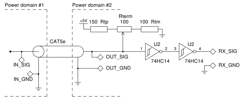
Figure 15. Signal recovery using the Schmitt trigger and separate power areas

Note:In the circuit in Figure 15, two inverters are used only to save the phase of the signal.

The signal at the cable exit must be “raised” to match the voltage levels for “0” and “1”. This is done by adjusting the Rterm resistor so that the bias voltage at the cable output is somewhere in the middle between the Schmitt trigger thresholds. The threshold voltages for 74HC14 when powered from 5 V are equal: V _{T +} = 2.4 V, V _T- = 1.4 V.

It will be logical to set the divider to offset 1.9 V (midway between the thresholds), but this must be confirmed experimentally. A terminator with a setting of 1.9 V has a composite resistance of 82 Ohms, which is slightly less than the required one hundred, but still acceptable. The resistance of the power supply to the alternating current is very small, so we can assume that the upper and lower pins of the divider are interconnected by alternating current. From the point of view of the signal at the end of the cable, the upper and lower shoulders of the divider are connected in parallel . Offset 1.9 V correspond to the resistance of the shoulders: 217 ohms - to the power conductor and 133 ohms - to the ground.


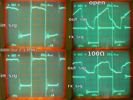
Figure 16. Signal recovery using level offset does not distort the pulse ratio

Returning to the second point, balancing the signal. Figure 16 (top right) shows what happens on the inconsistent line. The pulse duration from the source, 251.4 ns, is not equal to the duration at the output of the Schmitt trigger. The output pulse is 40 ns longer or nearly 16%. If you connect several transmission lines in a cascade, then just a few stages from the signal nothing remains (that is, the fill factor reaches 100% and the pauses between the pulses will disappear. - Approx. Transl. ) .

It is important to note that changes in the duty cycle strongly depend on the frequency of the signal and the length of the line. A small change in frequency may have a significant impact, while other changes may be invisible. The fact that the problem is not visible is not always a sign of the absence of a problem.

Adding a terminator with an offset (Fig. 16, bottom right) results in a perfect match of the pulse durations. To restore the duty cycle, the displacement level is set at 1.81 V (instead of the theoretical 1.9 V). Perhaps this is due to a small deviation of resistance from the nominal.

In real life, you would perform several construction tests, and then recalculate all the values ​​to make sure they are correct. Nobody needs trimming resistors in the final design, but they are usually not required. Most schemes, if properly designed, work normally with deviations within a few percent.

Resonance effects

Reflections in a long line can cause significant problems if the input wavelength is a multiple of the cable length. Figure 17 shows the waveforms of signals for a set of frequencies for which the 80-meter cable is 1/8 λ, 1/4 λ, 1/2 λ, 3/4 λ, and 1 λ.

As mentioned above, the first resonance occurs in the 1/4 λ mode. However, a standing wave occurs if any integer quarter- wave is placed on the line . At the end of the cable there will be an antinode of the wave if an odd number of quarter-waves (1/4 λ, 3/4 λ ...) fits into the line, and a wave node - if even (1/2 λ, 1 λ ...). (Here we are talking about nodes and voltage antinodes. The current wave is shifted by 1/4 λ relative to the voltage wave, i.e. the voltage antinodes correspond to the current node and vice versa. -Note trans. )

The problem arises when there is an antinode voltage at the end of the cable. The output voltage is a superposition of the input and voltage of the resonant wave. The amplitude of the voltage wave strongly depends on the quality factor (Q) of the cable. The quality factor, in turn, is determined by the resistance, capacitance and inductance of the line. At high values ​​of Q (Q> 1), the voltage at the antinode of the standing wave can significantly exceed the input voltage.

In the field of high-power radio signals, there are known cases of cable damage by a resonant wave. The voltage in the antinodes reached such values ​​that punched the cable insulation.


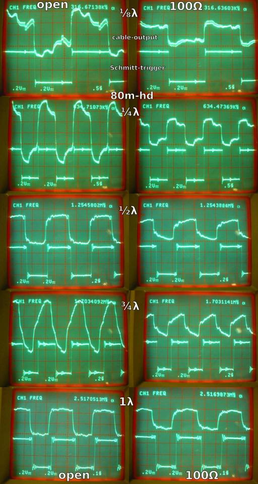
Figure 17. Resonant effects at different frequencies. On the left, the nonterminated line, on the right, the terminated line. The upper channel of the oscilloscope is the line output, the lower is the recovered signal.

The frequency of the resonant wave, for which the line length is equal to λ, can be found on the basis of the magnitude of the transmission delay. The measured delay is 402 ns, which gives a frequency of about 2.5 MHz. Figure 17 (bottom row) shows this frequency, within the margin of error.

It should be noted that the line becomes “transparent” when its length is a multiple of the wavelength (that is, the input impedance of the line will be equal to the load resistance, and will not depend on the characteristic impedance of the line. - Approx. Transl. ) . In this case, the capacitive and inductive components compensate each other.

Looking at Figure 17, it can be said that signal recovery works exceptionally reliably. However, you should not expect that your equipment will live for a long time if it is forced to cope with high voltage at the cable outlet.

Line Inlet Matching

The long lines are symmetrical in nature. From the point of view of coordination, this means: what was said about the line exit is also true for the entrance. Correct line matching is as follows:

1. the output impedance of the source is equal to the characteristic impedance of the line;
2. characteristic impedance is constant along the entire length of the line;
3. load resistance (terminator) is equal to wave resistance.

Until now, only the implementations of points 2 and 3 have been considered. Nevertheless, it is possible to create a system for which only items 1 and 2 are executed.


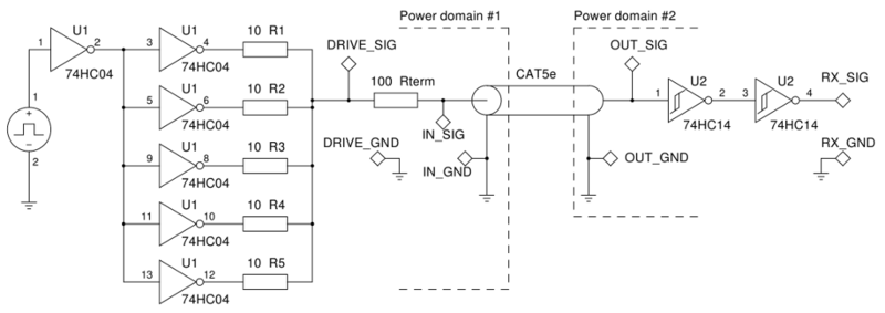
Figure 18. The high-current power supply circuit with consistent matching

The signal source (74HC04 buffers) has a very low output resistance (less than 5 ohms). The 100-ohm series-connected resistor Rterm matches the source impedance with the line impedance.


Figure 19. Sequential matching at the line input

When a signal is sent to the cable, it is reflected from the output and moves back to the beginning of the line. Since the input is properly matched, all energy leaves the cable without multiple reflections. In Figure 19 it can be seen that the reflection is superimposed on the useful signal only at the point IN_SIG and nowhere else.

There is no resonance in the cable, since there are no conditions for multiple signal reflections. Thus, the output voltage is always stable.

The main advantage of this scheme is its simplicity. The second advantage is that energy consumption is reduced. The driver is always loaded with a resistance of 100 Ohms, which limits the peak current to 50 mA (at 5 V). However, power reduction is also a disadvantage, since it does not allow you to quickly “shake” the cable capacity. This means that the bandwidth of the line will be limited.

Another disadvantage of this circuit is that the line driver must have a low output impedance and cope with the reflected signal. In practice, protective diodes may be required to limit overvoltages.

A few notes about the solution described:

• load resistance should be much greater than the line impedance. This is important because the reflection of the signal is artificially caused. When using the Schmitt trigger (Figure 18), this does not cause difficulties. Too low a load resistance (but still above the wave resistance) affects the desired value of the terminating resistor;
• You can balance the output of the cable with a high impedance divider;
• this installation does not resolve land allocation issues, as discussed earlier, and you must solve them separately;
• The installation is not insured against problems occurring near resonant frequencies.

Bilateral negotiation

As follows from the theory, and as described in the previous paragraph, the line should be consistent at the beginning and at the end. Why not do it?

Additional resistance makes signal recovery challenging. It has already been said that 80 meters of cable with a 100-ohm terminator will give a maximum output voltage of just 3.85 V due to the effect of a voltage divider. The introduction of an additional resistor at the beginning of the cable for matching on both sides will reduce the output voltage to 5 V · 100 Ohms / (100 Ohms + 100 Ohms + 30 Ohms) = 2.17 V. With such an amplitude, the Schmitt trigger threshold (2.4 B) will never be reached, and the signal will disappear.

A short cable will give you 2.5 V at best, which does not leave a large margin for stable operation.

Transmitting a digital signal requires that the minimum amplitude at the cable's output comply with the specification. There is no other way to achieve this, except for the use of additional circuits for signal amplification.

Isolation of power

Several times in this article the problem of earthen loops was emphasized. The creation of short circuits in the conductors of the earth can lead to an uncontrolled "ringing" at different frequencies. Unfortunately, this problem is simply formulated, but does not have a simple solution.

The best solution is to ensure that the earth's conductors cannot connect, even through the hull, screen, or external ground. However, this solution is not always practical, and, of course, not cheap. There is a fairly simple way to untie power supplies, along with their lands, when power is connected in conjunction with connecting signal circuits.


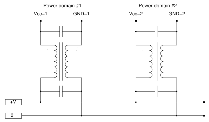
Figure 20. Isolation of power with chokes

Each power line branch passes through the choke (or ferrite bead). Both wires, positive and negative, must be twisted together. The windings on the choke are wound in such a way that the magnetic fields of the positive and negative conductors compensate each other and permanent bias is not created.

A choke exerts a very large resistance to differential variable signals, and this ensures that the common wire of a long line, on which a variable signal is present, has no connection to the power buses. Capacitors on each side of the choke, which have a low impedance at high frequency, allow each supply area to be considered as a local, isolated source (alternating current).

The required inductance of chokes and capacitor capacitance will depend on the frequency of the transmitted signals. Lower frequencies mean using higher values. It completely depends on the design as a whole.

The power line separation shown in Figure 20 does not provide a perfect isolation of the ground. For example, the resistance of a ground conductor for direct current will still depend on the layout of the earth. Changing this resistance will change the parameters of the voltage divider and shift the absolute levels of the signals, but this should not cause any special problems, and sometimes it can even be useful.

Balance lines

Instead of using complicated ground layouts, you can simply stop using the ground as a point of reference, and leave signal levels floating freely.

Denial of the common wire as a zero level is accomplished by applying “positive” and “negative” connections between the source and the receiver. The signal is encoded by the potential difference between the "+" and "-" conductors, without taking into account the absolute value of these potentials. Such a system is called a differential pair .

Examples of balanced transmission lines are RS-485 , CAN , USB and LVDS .

Balance lines do not solve all the problems associated with long lines. They still need to be properly coordinated, like other cables. However, the advantages of balanced lines include very good noise immunity, the absence of a common wire and a wide bandwidth. The price for this is the complication of the receiver-transmitter circuits.

Conclusion

You can still tell a lot on the topic of data lines. Written many books about the intricacies of the cables and long lines. I hope you were able to sort out some issues with the help of the examples given. A few tips on the design of transmission lines for your future development:

• make sure the signals are transmitted correctly and not reflected;
• do not forget to put terminators;
• if the driver can withstand the reflected signal, put a terminator at the line input;
• if reflections are undesirable, terminate the end of the line;
• check the power circuit and exclude ground loops;
• at high frequencies it is better to use balanced lines and specialized drivers;
• if something is beyond your comprehension, consult with experts.

May the Force be with you!