I do not know about you, dear reader, but I have always been amazed at the contrast between the grace of the basic idea embedded in the concept of binary search trees and the complexity of implementing balanced binary search trees ( red-black trees , AVL-trees , Cartesian trees ). Recently, turning over Sedgwick [ 1 ] once again, I found a description of randomized search trees (the original work [ 2 ] was also found) - so simple that it only takes a third of a page (insert nodes, another page delete nodes). In addition, upon closer inspection, an additional bonus emerged in the form of a very beautiful implementation of the operation of removing nodes from the search tree. Below you will find a description (with color pictures) of randomized search trees, implementation in C ++, as well as the results of a small author's study of the balance of the described trees.

Start little by little

Since I am going to describe the full implementation of the tree, I will have to start from the beginning (professionals can easily skip a couple of sections). Each node of the binary search tree will contain a key key, which essentially controls all processes (we will have it intact), and a pair of left and right pointers to the left and right subtrees. If any pointer is zero, then the corresponding tree is empty (i.e., simply absent). In addition to this, we will need another size field to implement a randomized tree, which will store the size (in parrots tops) of the tree with the root in this node. Nodes will be represented by structures:

struct node //      { int key; int size; node* left; node* right; node(int k) { key = k; left = right = 0; size = 1; } };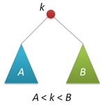 

The main property of the search tree is that any key in the left subtree is smaller than the root key, and in the right subtree it is larger than the root key (for clarity, we will assume that all keys are different). This property (shown schematically in the figure on the right) allows us to very simply organize the search for a given key, moving from the root to the right or left depending on the value of the root key. The recursive version of the search function (and we will consider only such) looks like this:

 node* find(node* p, int k) //   k   p { if( !p ) return 0; //       if( k == p->key ) return p; if( k < p->key ) return find(p->left,k); else return find(p->right,k); } 

Go to insert new keys in the tree. In the classic version of the insert repeats the search with the difference that when we run into a null pointer, we create a new node and hang it to the place where we found a dead end. At first, I did not want to paint this function, because in the randomized case it works a little differently, but changed my mind, because I want to fix a couple of moments.

 node* insert(node* p, int k) //       k   p { if( !p ) return new node(k); if( p->key>k ) p->left = insert(p->left,k); else p->right = insert(p->right,k); fixsize(p); return p; } 

First, any function that modifies a given tree returns a pointer to a new root (whether it has changed or not), and then the caller itself decides where to hang the tree. Secondly, because we have to keep the size of the tree, then for any change of subtrees we need to adjust the size of the tree itself. The following pair of functions will do this for us:

 int getsize(node* p) //    size,     (t=NULL) { if( !p ) return 0; return p->size; } void fixsize(node* p) //     { p->size = getsize(p->left)+getsize(p->right)+1; } 

What is wrong with the insert function? The problem is that this function does not guarantee the balance of the resulting tree, for example, if the keys are given in ascending order, the tree will degenerate into a single-linked list (see figure) with all the accompanying "buns", the main of which is the linear execution time all operations on such a tree (while for balanced trees this time is logarithmic). There are various ways to avoid imbalance. Conventionally, they can be divided into two classes, those that guarantee balance (red-black trees, AVL-trees), and those that provide it in a probabilistic sense (Cartesian trees) - the probability of obtaining an unsubstituted tree is negligible for large tree sizes. I think it will not be a surprise if I say that randomized trees belong to the second class.

Insert in the root of the tree

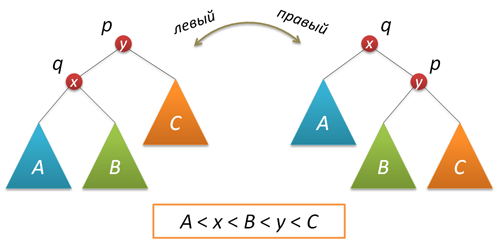
A necessary component of randomization is the use of a special insert of a new key, as a result of which a new key appears at the root of the tree (a useful function in many ways, since access to recently inserted keys turns out to be very fast, hello to self-organizing lists ). To implement the insert into the root, we need a rotation function that performs a local transformation of the tree.


')
Do not forget to adjust the size of the subtrees and return the root of the new tree:

 node* rotateright(node* p) //     p { node* q = p->left; if( !q ) return p; p->left = q->right; q->right = p; q->size = p->size; fixsize(p); return q; } 

 node* rotateleft(node* q) //     q { node* p = q->right; if( !p ) return q; q->right = p->left; p->left = q; p->size = q->size; fixsize(q); return p; } 

Now actually insert into the root. First, we recursively insert the new key into the root of the left or right subtree (depending on the result of the comparison with the root key) and perform a right (left) turn, which raises the node we need to the root of the tree.

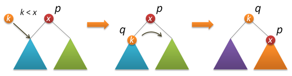
 node* insertroot(node* p, int k) //      k    p { if( !p ) return new node(k); if( k<p->key ) { p->left = insertroot(p->left,k); return rotateright(p); } else { p->right = insertroot(p->right,k); return rotateleft(p); } } 

Randomized insert

So we got to randomization. At this moment we have two insertion functions - a simple one and a root, of which we now combine the randomized insert. The meaning of all this lies in the following idea. It is known that if you mix all the keys in advance and then build a tree out of them (the keys are inserted according to the standard scheme in the order obtained after mixing), then the tree will be well balanced (its height will be about 2log ₂ n versus log ₂ n for perfectly balanced tree). Note that in this case any of the original keys can be with the same probability as the root. What to do if we do not know in advance what keys we will have (for example, they are entered into the system when using the tree)? In fact, everything is simple. Since any key (including the one that we now have to insert into the tree) can turn out to be a root with probability 1 / (n + 1) (n is the size of the tree before insertion), then we perform with the specified probability an insert into the root, and with probability 1-1 / (n + 1) - recursive insertion into the right or left subtree depending on the key value in the root:

 node* insert(node* p, int k) //       k   p { if( !p ) return new node(k); if( rand()%(p->size+1)==0 ) return insertroot(p,k); if( p->key>k ) p->left = insert(p->left,k); else p->right = insert(p->right,k); fixsize(p); return p; } 

That's the whole trick ... Let's see how it all works. An example of building a tree of 500 nodes (the keys from 0 to 499 were received at the entrance in ascending order):
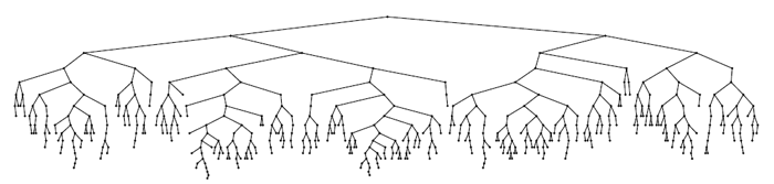Not to say that the ideal of beauty, but the height is clearly small. Let's complicate the task - we will build a tree, giving the input keys from 0 to 2 ¹⁴ -1 (the ideal height is 14), and measure the height in the construction process. For reliability, we will do a thousand runs and average the result. We obtain the following graph, in which our results are marked with markers, and the solid line from the theoretical estimate from [ 3 ] is h = 4.3ln (n) -1.9ln (ln (n)) -4. The most important thing that we see from the figure is that probability theory is power!

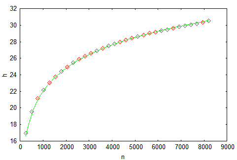
It should be understood that the proposed graph shows the average height of the tree by a large number of calculations. And how much height can differ in one particular calculation. The above article has an answer to this question. We will act on workers and peasants and build a histogram of the distribution of heights after the insertion of 4095 nodes.

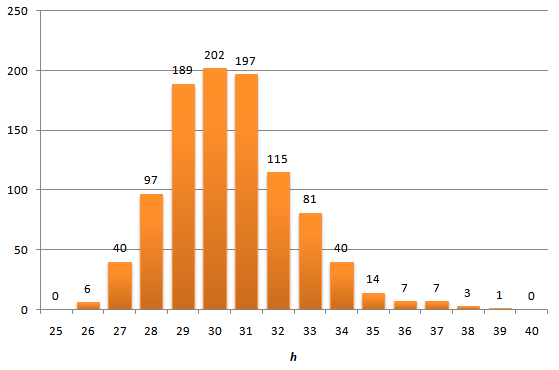
In general, no crime is visible, the distribution tails are short - the maximum height obtained is 39, which is not much higher than the hospital average.

Deleting keys

So, we have a balanced (at least in some sense) tree. True, while it does not support the removal of nodes. This is what we will do now. The removal option, which is prescribed in many textbooks and which is well (with pictures) described on Habré , can and works quickly, but it looks very unrepresented (compared to the insert). We will go the other way, approximately as it was shown in this wonderful post (in my opinion, this is the best description of Cartesian trees). Before removing the nodes, learn how to connect the trees. Let two search trees with roots p and q be given, and any key of the first tree is less than any key in the second tree. It is required to combine these two trees into one. As the root of a new tree, you can take either of the two roots, let it be p. Then the left subtree p can be left as it is, and on the right p hang up the union of two trees - the right subtree p and the whole tree q (they satisfy all the conditions of the problem).

On the other hand, with the same success, we can make the root of the new tree node q. In a randomized implementation, the choice between these alternatives is made randomly. Let the size of the left tree be n, the right one - m. Then p is chosen as the new root with probability n / (n + m), and q with probability m / (n + m).

 node* join(node* p, node* q) //    { if( !p ) return q; if( !q ) return p; if( rand()%(p->size+q->size) < p->size ) { p->right = join(p->right,q); fixsize(p); return p; } else { q->left = join(p,q->left); fixsize(q); return q; } }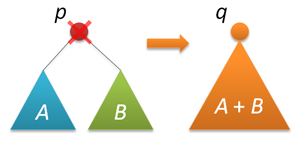 

Now everything is ready for removal. We will delete by key - we look for the node with the given key (I remind you that we have all the keys are different) and remove this node from the tree. The search stage is the same as in the search (oddly enough), but then we do it further - we merge the left and right subtrees of the found node, delete the node, return the root of the merged tree.

 node* remove(node* p, int k) //    p      k { if( !p ) return p; if( p->key==k ) { node* q = join(p->left,p->right); delete p; return q; } else if( k<p->key ) p->left = remove(p->left,k); else p->right = remove(p->right,k); return p; } 

We verify that deletion does not disturb the balance of the tree. To do this, we will build a tree with 2 ¹⁵ keys, then delete half (with values ​​from 0 to 2 ¹⁴ -1) and look at the distribution of heights ...

Virtually no difference, as required to "prove" ...

Instead of conclusion

The undoubted advantage of randomized binary search trees is the simplicity and beauty of their implementation. However, as you know free cakes do not happen. What are we paying in this case? First, additional memory for storing subtree sizes. One integer field per node. With some dexterity, red-and-black trees can do without additional fields. On the other hand, the size of the tree is not completely useless information, because it allows you to organize access to data by number (the task of sampling or search for ordinal statistics), which turns our tree, in fact, into an ordered array with the ability to insert and delete any elements. Secondly, the operation time is logarithmic, but I suspect that the proportionality constant will be rather big - almost all operations are performed in two passes (and down and up), besides, insertion and deletion require random numbers. There is good news - at the search stage everything should work very quickly. Finally, the principal obstacle to using such trees in serious applications is that logarithmic time is not guaranteed; there is always a chance that the tree will turn out to be poorly balanced. True, the probability of such an event already at ten thousand knots is so small that, perhaps, you can take a risk ...

Thanks for attention!

Literature

1. Robert Sedgwick, Algorithms in C ++, M .: Williams, 2011 - just a good book
2. Martinez, Conrado; Roura, Salvador (1998), ACM (ACM Press) 45 (2): 288–323 - original article
3. Reed, Bruce (2003), The ACM 50 (3): 306–332 - a binary tree search