Algorithm for modeling a multidimensional array of data distributed according to the normal law
When developing or researching ready-made algorithms, it is often required to determine the quality of their work. It is not always possible to use data from real sources for this purpose, since their properties are often unknown and therefore it is impossible to predict the result of the execution of the investigated algorithms. In this case, data modeling using one of the well-known distribution laws is used. Applying the studied algorithm to the model data, it is possible to assume in advance what the result of its implementation will be. If it is satisfactory, you can try to apply it to real data. Naturally, this applies only to non-parametric algorithms, that is, independent of the data distribution law.
The most commonly used data modeling is distributed according to the normal law. Unfortunately, MS Excel and common statistical packages (SPSS, Statistica) allow to model only one-dimensional statistical distributions. Of course, you can make a multidimensional distribution of several one-dimensional, but only if the variables are independent. If you need to investigate data with variables dependent on each other, you will have to write a program.
Usually indicate that the multidimensional normal distribution described by the vector of mathematical expectations
  and positively defined covariance matrix
  :
:

where ;
;
i = 1,2,3, ... m, j = 1,2,3, ..., m;
m is the number of signs of a multidimensional normal sample.
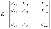
However, instead of the covariance matrix, it is more convenient to use the correlation matrix. and dispersion vector
  because the correlation coefficient shows the degree of connection between variables, in contrast to the covariance coefficient. The correlation matrix is:

')
Transform matrix coefficients to matrix coefficients
  occurs according to the formula:

To model the vector linear vector transform can be used
  whose components are normally distributed random variables with the parameters of the expectation equal to zero and the variance equal to one (i.e.
  ). To simulate a one-dimensional normal random variable, there are many ways, for example, the Box-Muller transform: using two random numbers
  and
and  distributed on the interval (0; 1], at which two numbers are obtained simultaneously, distributed according to the normal law with parameters
  :
:


Transformation at
at  produced by the formula:

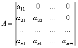
In this conversion there is a lower triangular matrix that derives from the matrix
  Cholesky decomposition
  :
:

Each element of the matrix determined by a recurrent procedure:

where indexes vary in range , and the sums with the upper zero limit are equal to zero (that is, if
  then
then  ,
,  ).
).
The described transformation can be implemented as two functions in C ++: the main function normal_model (), which implements the algorithm and the auxiliary matrix_determinant (), which returns the determinant of the matrix.
The normal_model () function determines the number of required variables and values from the dimension of the matrix with the result. Returns true on success, false on failure.
The result of the work can be found here . The function is accessed via the fastcgi mechanism.
Used Books:
The most commonly used data modeling is distributed according to the normal law. Unfortunately, MS Excel and common statistical packages (SPSS, Statistica) allow to model only one-dimensional statistical distributions. Of course, you can make a multidimensional distribution of several one-dimensional, but only if the variables are independent. If you need to investigate data with variables dependent on each other, you will have to write a program.
Usually indicate that the multidimensional normal distribution
 described by the vector of mathematical expectations
  and positively defined covariance matrix
  :
:
where
 ;
;i = 1,2,3, ... m, j = 1,2,3, ..., m;
m is the number of signs of a multidimensional normal sample.
However, instead of the covariance matrix, it is more convenient to use the correlation matrix.
 and dispersion vector
  because the correlation coefficient shows the degree of connection between variables, in contrast to the covariance coefficient. The correlation matrix is:
')
Transform matrix coefficients
 to matrix coefficients
  occurs according to the formula:
To model the vector
 linear vector transform can be used
  whose components are normally distributed random variables with the parameters of the expectation equal to zero and the variance equal to one (i.e.
  ). To simulate a one-dimensional normal random variable, there are many ways, for example, the Box-Muller transform: using two random numbers
  and
and  distributed on the interval (0; 1], at which two numbers are obtained simultaneously, distributed according to the normal law with parameters
  :
:

Transformation
 at
at  produced by the formula:
In this conversion
 there is a lower triangular matrix that derives from the matrix
  Cholesky decomposition
  :
:
Each element of the matrix
 determined by a recurrent procedure:
where indexes vary in range
 , and the sums with the upper zero limit are equal to zero (that is, if
  then
then  ,
,  ).
).The described transformation can be implemented as two functions in C ++: the main function normal_model (), which implements the algorithm and the auxiliary matrix_determinant (), which returns the determinant of the matrix.
The normal_model () function determines the number of required variables and values from the dimension of the matrix with the result. Returns true on success, false on failure.
// , . //double MatrixMath [mq] - . //double MatrixDisp [mq] - //vector<vector<double> > &correlation_matrix - //vector<vector<double> > &MatrixRes - bool normal_model (double MatrixMath[], double MatrixVar[], vector<vector<double> > &correlation_matrix, vector<vector<double> > &MatrixRes){ int mq =MatrixRes[0].size();// int count=MatrixRes.size();// double MatrixA[mq][mq]; // A double MatrixN[count][mq]; // , 0, 1 int i,j,k; double suma, sumaa; double alfa1, alfa2; //. , (0;1] vector<vector<double> > MatrixK(mq); // K for (i=0;i<mq;i++){ MatrixK[i].resize(mq); } // for (i=0; i<mq; i++){ for (j=0; j<mq; j++){ MatrixK[i][j]= correlation_matrix[i][j]* sqrt(MatrixVar[i]*MatrixVar[j]); } } if (matrix_determinant(MatrixK)<=0) return false; // . ; // A for (i=0; i<mq; i++){ for (j=0; j<=i; j++){ sumA=0; sumAA=0; for (k=0; k<j; k++){ sumA+= MatrixA[i][k] * MatrixA[j][k]; sumAA+= MatrixA[j][k] * MatrixA[j][k]; } MatrixA[i][j]=(MatrixK[i][j] - sumA)/ sqrt(MatrixK[j][j] - sumAA); } } // , 0, 1 srand(time(NULL)); for (i=0; i<count; i+=2){ for (j=0; j<mq; j++){ alfa1 = (double)rand()/(RAND_MAX+1.0); alfa2 = (double)rand()/(RAND_MAX+1.0); if (!alfa1 || !alfa2){ j--; }else{ MatrixN[i][j] = sqrt(-2*log(alfa1))*sin(2*M_PI*alfa2); if (i+1<count) MatrixN[i+1][j] = sqrt(-2*log(alfa1))*cos(2*M_PI*alfa2); } } } // , 0, 1 for (i=0; i<count; i++){ for (j=0; j<mq; j++){ MatrixRes[i][j]=MatrixMath[j]; for (k=0; k<mq; k++){ MatrixRes[i][j]+=MatrixA[j][k] * MatrixN[i][k]; } } } return true; } // m N x N double matrix_determinant (vector<vector<double> > & m){ double result=0; if (m.size()==1){ return m[0][0]; }else if(m.size()==2){ return m[0][0] * m[1][1] - m[0][1] * m[1][0]; }else if(m.size()==3){ return m[0][0] * m[1][1] * m[2][2] + m[0][1] * m[1][2] * m[2][0] + m[0][2] * m[1][0] * m[2][1] - m[2][0] * m[1][1] * m[0][2] - m[1][0] * m[0][1] * m[2][2] - m[0][0] * m[2][1] * m[1][2]; }else{ vector<vector<double> > m1(m.size()-1);// N-1 x N-1, N-1 for (int i=0; i<m.size()-1; i++){ m1[i].resize(m.size()-1); } for (int i=0; i< m.size(); i++){ for (int j=1; j<m.size(); j++){ for (int k=0; k<m.size(); k++){ if (k<i){ m1[j-1][k] = m[j][k]; }else if(k>i){ m1[j-1][k-1] = m[j][k]; } } } result+= pow(-1,i) *m[0][i] * matrix_determinant(m1); } } return result; } The result of the work can be found here . The function is accessed via the fastcgi mechanism.
Used Books:
- Martyshenko S.N., Martyshenko N.S., Kustov D.A. Simulation of multidimensional data and computer experiment. Technique and technology, 2007. - №2. Pp. 47–52.
- Ermakov SM, Mikhailov GA, Statistical modeling. M .: Nauka, 1982.
- V. Feller, Introduction to Probability Theory and Its Applications, trans. from English, t. 1-2, M., 1964-67.
- Rencher, Alvin C. (2002), Methods of Multivariate Analysis, Second Edition, John Wiley & Sons.
Source: https://habr.com/ru/post/145315/
All Articles