Risk calculation by Value at Risk

The last decades the world economy regularly falls into the maelstrom of financial crises. 1987, 1997, 2008 nearly led to the collapse of the existing financial system, which is why leading experts began to develop methods, with the help of which one can control the uncertainty prevailing in the financial world. In the Nobel Prizes of recent years (obtained for the Black-Scholes model, VaR, etc.) there is a clear tendency towards mathematical modeling of economic processes, attempts to predict market behavior and assess its stability.

Today I will try to talk about the most widely used method for predicting losses - Value at Risk (VaR).

VaR concept

The VaR 's explanation, clear to the economist, is as follows: “Estimate, expressed in monetary units, of a value that will not exceed the expected loss during a given period of time with a given probability.” In essence, VaR is the amount of losses in an investment portfolio for a fixed period of time, in case some unfavorable events happen. By “not favorable events” one can understand various crises, poorly predictable factors (changes in legislation, natural disasters, ...) that can affect the market. As a time horizon, usually choose one, five or ten days, due to the fact that for a longer period to predict market behavior is extremely difficult. The level of acceptable risk (in essence, the confidence interval) is taken to be 95% or 99%. Also, of course, the currency is fixed in which we will measure losses.
When calculating the value, it is assumed that the market will behave in a “normal” manner. Graphically, this value can be illustrated as follows:


')

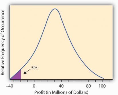
VaR calculation methods

Consider the most commonly used methods for calculating VaR, as well as their advantages and disadvantages.

Historical modeling

In historical modeling, we take the values ​​of financial fluctuations for the portfolio already known from past measurements. For example, we have portfolio behavior over the previous 200 days, on the basis of which we decide to calculate VaR. Suppose that the next day the financial portfolio will behave in the same way as in one of the previous days. So we get 200 outcomes the next day. Further, we assume that the random variable is distributed according to the normal law, based on this fact, we understand that VaR is one of the percentiles of the normal distribution. Depending on what level of acceptable risk we have taken, we select the corresponding percentile and, as a result, we get the value we are interested in.

The disadvantage of this method is the impossibility of constructing predictions for portfolios about which we have no information. There may also be a problem if the components of the portfolio change significantly in a short period of time.

A good example of calculations can be found at the following link .

Leading component method

For each financial portfolio, you can calculate a set of characteristics that help assess the potential of assets. These characteristics are called leading components and usually represent a set of partial derivatives of the price of a portfolio. To calculate the value of a portfolio, the Black-Scholes model is usually used, which I will try to describe next time. In a nutshell, a model is a dependence of a European option on time and its current value. Based on the behavior of the model, we can estimate the potential of an option by analyzing the function using classical methods of mathematical analysis (convexity / concavity, intervals of increase / decrease, etc.). Based on the analysis data, the VaR are calculated for each of the components and the resulting value is plotted as a combination (usually a weighted sum) of each of the estimates.

Monte Carlo method

The Monte Carlo method is in many ways similar to the method of historical modeling, the difference is that the calculation is not based on real data, but on randomly generated values. The advantage of this method is the ability to consider as a large number of situations, and emulate market behavior in extreme conditions. The obvious drawback is the large computational resources required to implement this approach. When working with this technique, NoSQL storage and distributed computing based on MapReduce are commonly used. A good example of using Hadoop to calculate VaR can be found at the following link .

Naturally, these are not the only methods for calculating VaR. There are both simple linear and quadratic models of price prediction, and a rather complicated method of variations, covariances, which I have not mentioned, but those interested can find a description of the techniques in the books below.

Criticism of the technique

It is important to note that when calculating VaR, the hypothesis of normal market behavior is accepted; however, if this assumption were correct, crises would occur every seven thousand years, but, as we see, this is absolutely not true. Nassim Taleb, a well-known trader and mathematician, in the books Frowned by Accident and Black Swan, exposes the existing risk assessment system to harsh criticism, and also offers his solution in the form of using another risk calculation system based on the log-normal distribution.

Despite criticism, VaR is quite successfully used in all major financial institutions. It should be noted that this approach is not always applicable, which is why other techniques were created with a similar idea, but a different method of calculation (for example, SVA).

Taking into account the criticism, VaR modifications were developed, based either on other distributions or on other methods of calculation on the peak of the Gaussian curve. But I will try to tell about this another time.

Links

Several interesting books on the topic:

• Options, futures and other derivative financial instruments
• Black Swan. Under the sign of unpredictability
• Fooled by randomness. About the hidden role of chance in business and in life