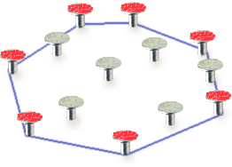
Having conducted a small scientific study (in other words, by performing a search on the site), I found out that there are only two articles with the tag “ computational geometry ,” and one of them turned out to be mine. Because Recently, I have become somewhat interested in this topic, I decided to continue the topic of algorithmic geometry with the consideration of the problem of constructing the so-called minimal convex hulls . Although the figure on the right gives an insightful hackleader an exhaustive explanation of what it is, nevertheless, a bit more formal definitions will be given under the cut and two classical algorithms for constructing minimal convex hulls will be described.

The concept of a minimal convex hull

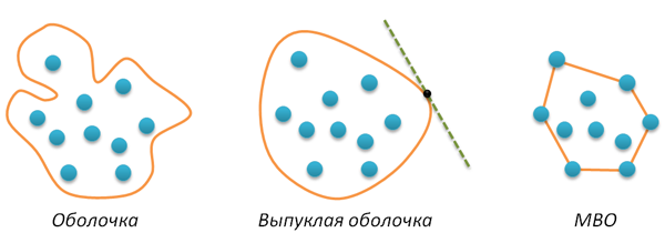
Let a finite set of points A be given on a plane. A shell of this set is any closed line H without self-intersections such that all points of A lie inside this curve. If the curve H is convex (for example, any tangent to this curve does not intersect it at any other point), then the corresponding envelope is also called convex . Finally, the minimal convex hull (hereinafter briefly MBO) is the convex hull of minimal length (minimal perimeter). I did not check (it seems that this can be proved by contradiction), but it seems obvious that the minimal hull simply must be convex. All introduced concepts are illustrated by the following figure.

The main feature of the MVO of the set of points A is that this shell is a convex polygon whose vertices are some points of A. Therefore, the task of finding the MVO ultimately reduces to selecting and ordering the necessary points from A. Ordering is necessary for the reason that the output of the algorithm should be a polygon, i.e. sequence of vertices. We additionally impose a condition on the order of the vertices - the direction of the polygon traversal must be positive (I remind you that a counterclockwise figure traversal is called positive).

The task of building an MVO is considered one of the simplest tasks of computational geometry, for it there are many different algorithms. Below we consider two such algorithms - Graham scan and Jarvis march. Their description is illustrated with a Python code. Both algorithms will need the rotate function, described in detail in my previous post . Recall that this function determines which side of the vector AB is the point C (positive return value corresponds to the left side, negative - the right side).

def rotate(A,B,C): return (B[0]-A[0])*(C[1]-B[1])-(B[1]-A[1])*(C[0]-B[0]) 

')

Graham scan algorithm

This algorithm is a three-step. At the first step, any point in A that is guaranteed to be included in the MBO is searched. It is easy to figure out that such a point will be, for example, a point with the smallest x-coordinate (the leftmost point in A). This point (we will call it the starting point) is moved to the top of the list, all further work will be done with the remaining points. For some reasons, we will not change the initial array of points A, for all manipulations with points we will use indirect addressing: we will get a list of P in which numbers of points will be stored (their positions in array A). So, the first step of the algorithm is that the first point in P should be the point with the smallest x-coordinate. Code:

 def grahamscan(A): n = len(A) #   P = range(n) #    for i in range(1,n): if A[P[i]][0]<A[P[0]][0]: #  P[i]-    P[0]-  P[i], P[0] = P[0], P[i] #      

The second step in Graham’s algorithm is the sorting of all points (except P [0] -th), according to the degree of their left-handedness relative to the starting point R = A _{P [0]} . We say that B <C if the point C is on the left side of the RB vector.

To perform such ordering, you can use any sorting algorithm based on pairwise comparison of elements, for example, quick sorting. For some reason (the main one is clumsiness of hands), I will use sorting by inserts.
* _{I will be very grateful to those who can explain to me how to apply in this case the built-in Python sorting ...}
So, sorting by inserts (do not forget about indirect addressing and the fact that the zero point is not sorted):

  for i in range(2,n): j = i while j>1 and (rotate(A[P[0]],A[P[j-1]],A[P[j]])<0): P[j], P[j-1] = P[j-1], P[j] j -= 1 

The result of sorting can be illustrated by the following figure.

If we now connect the points in the order obtained, we obtain a polygon, which, however, is not convex.

Moving on to the third action. All we have to do is cut the corners. To do this, go through all the vertices and remove those of them in which the right turn is performed (the angle at such a vertex turns out to be more unfolded). We get the stack S (really a list) and put the first two vertices into it (again, they are guaranteed to be included in the MBO).

  S = [P[0],P[1]] 

Then we look through all the other vertices, and track the direction of rotation in them from the point of view of the last two vertices in the S stack: if this direction is negative, then we can cut off the angle by removing the last vertex from the stack. As soon as the turn turns out to be positive, the cutting of the corners is completed, the current vertex is pushed onto the stack.

  for i in range(2,n): while rotate(A[S[-2]],A[S[-1]],A[P[i]])<0: del S[-1] # pop(S) S.append(P[i]) # push(S,P[i]) 

As a result, the required sequence of vertices appears in the stack S (which can now be considered as a list), and in the orientation we need, defining the MBO of a given set of points A.

  return S 

The complexity of the first and last steps of the algorithm is linear in n (although in the latter case there is an embedded loop, however, each vertex inside this cycle is pushed onto the stack exactly once, and not more than once removed from there), therefore, the complexity of the entire algorithm is determined by the second step - sorting, which is why insertion sorting is not the best option for large n. If we replace it with a quick sort, we obtain the total complexity of the algorithm O (nlogn). Is it possible to improve this time? If the algorithm is based on pairwise comparison of points (like ours), then it is proved that this estimate is generally not improved. From this point of view, Graham’s algorithm is optimal. Nevertheless, it does not have a very good feature - it is not adaptive in the sense that it does not matter how many vertices will eventually go into the MBO (three, five, ten, or n), all the same time will be linear logarithmic. Jarvis has such adaptability, to the consideration of which we smoothly proceed.

Jarvis Algorithm

The Jarvis algorithm (another name is the gift wrapping algorithm) is conceptually simpler than the Graham algorithm. It is a two-step and does not require sorting. The first step is exactly the same - we need a starting point, which is guaranteed to enter the MBO, take the leftmost point of A.

 def jarvismarch(A): n = len(A) P = range(n) for i in range(1,n): if A[P[i]][0]<A[P[0]][0]: P[i], P[0] = P[0], P[i] 

In the second step of the algorithm, an MBO is built. Idea: make the starting vertex current, look for the rightmost point in A relative to the current vertex, make it current, etc. The process ends when the starting vertex is current again. As soon as the dot hit the MVO, it can no longer be taken into account. Therefore, we will create another H list, in which the vertices of the MBO will be stored in the correct order. We immediately add the starting vertex to this list, and in the list P we transfer this vertex to the end (where we finally find it and complete the algorithm).

  H = [P[0]] del P[0] P.append(H[0]) 

Now we organize an infinite loop, at each iteration of which we look for the leftmost point from P with respect to the last vertex in H. If this vertex is the starting one, then we interrupt the cycle, if not, then we transfer the found vertex from P to H. After the completion of the cycle, the desired shell is in H which we return as a result.

  while True: right = 0 for i in range(1,len(P)): if rotate(A[H[-1]],A[P[right]],A[P[i]])<0: right = i if P[right]==H[0]: break else: H.append(P[right]) del P[right] return H 

Hmmm, I was able to talk about the Jarvis algorithm without using pictures. The following figure illustrates everything!

Estimate the complexity of the Jarvis algorithm. The first step is linear in n. With the second all the more interesting. We have a nested loop, the number of external iterations is equal to the number of vertices h in the MVO, the number of internal iterations does not exceed n. Therefore, the complexity of the entire algorithm is O (hn). Unusual in this formula is that the complexity is determined not only by the length of the input data, but also by the length of the output (output-sensitive algorithm). And then how the point cards will fall. In the worst case, all points from A enter the MBO (that is, A is a convex polygon by itself), then h = n and the complexity jumps to a quadratic one. At best (provided that the points of A do not lie on one straight line) h = 3 and the complexity becomes linear. It remains to understand in advance what our case is, what is not so easy to do (if you do not have a time machine ^** ), you can only proceed from the nature of the task - if there are a lot of points and they evenly fill a certain area, then Jarvis will be faster ( if the data is collected at the border area, then Graham will be faster, something like that ...
** _{The time machine is generally a useful thing from the point of view of algorithms, any task requiring a trillion years of computation can be solved almost instantly with its help - we start the program, sit in the time machine, “fly” to the future, read the result, go back. It remains to figure out how to ensure the uninterrupted operation of a computer for a couple of trillions of years ...}

Instead of conclusion

In my opinion, the task of constructing minimal convex hulls is a good way to get into the topic of computational geometry, it is easy enough to invent your own algorithm (however, it will most likely be a variation of the Jarvis algorithm). It is argued that there are many applications for this task, most of them are associated with pattern recognition, clustering, etc. In addition, the task of constructing an MVO is used as an aid in solving more complex problems of computational geometry. Yes, it is worth noting that this problem has a very interesting three-dimensional generalization.

Thank you all for your attention!