Forecasting financial time series

Introduction

Hello everyone, since a cycle of articles about neural networks has gone to Habre, then I will write about the possibility of using neural networks in the task of forecasting financial time series.
There are several different theories about the possibility of forecasting stock markets. One of them is the hypothesis of an effective market, according to her, the stock price has already taken into account all the available information and it makes no sense to make forecasts. The continuation of this hypothesis can be called the theory of random walks.
In the theory of random walks, information is divided into two categories - predictable, well-known and new, unexpected. If the predictable, and even more so already known information is already embedded in market prices, the new unexpected information in the price is not yet present. One of the properties of unpredictable information is its randomness and, accordingly, the randomness of the subsequent price change. The hypothesis of an effective market explains the change in prices by the arrival of new unexpected information, and the theory of random walks complements this with an opinion about randomness of price changes.

A brief practical conclusion of the theory of random walks - players are recommended to use the strategy of "buy and hold" in their work. It should be noted that the flourishing of the theory of random walks occurred in the 1970s, when the US stock market, traditionally the main testing ground for all new economic theories, did not show any obvious trends, and the market itself was in a narrow corridor. According to the hypothesis of an efficient market and the theory of random walks, price forecasting is impossible. ^[one]
However, the majority of market participants still use different methods for forecasting, suggesting that the series itself is full of hidden patterns.
Such hidden empirical patterns were attempted by the founder of technical analysis, R.Elliott, in his series of articles in the 1930s.
In the 1980s, this point of view found unexpected support in the theory of dynamic chaos that had just emerged. This theory is built on the opposition of randomness and stochasticity (randomness). Chaotic series only look random, but, as a deterministic dynamic process, they completely allow short-term forecasting. The area of ​​possible predictions is limited in time by the forecasting horizon, but this may be enough to generate real income from the predictions (Chorafas, 1994). And the one who has the best mathematical methods of extracting patterns from noisy chaotic series, can hope for a greater rate of return - at the expense of their less well-equipped counterparts. ^[2]

Forecasting methods

Currently, professional market participants use various methods for forecasting financial time series, the main ones are:
1) expert forecasting methods.
The most common method from the group of expert methods is the Delphi method. The essence of the method is to collect the opinions of various experts and their generalization into a single assessment. If we forecast financial markets with this method, then we need to select an expert group of people versed in this subject area (this could be analysts, professional traders, investors, banks, etc.), conduct a survey or survey and make a generalization of the current market situation.
2) Methods of logical modeling.
Based on the search and identification of market patterns in the long term.
These include methods:
- the method of scenarios ("if-then"), the description of sequences of outcomes from this or that event, with the creation of a knowledge base;
- methods of forecasts in the image;
- the method of analogies.
3) Economic and mathematical methods.
Methods from this group are based on the creation of models of the object under study. The economic-mathematical model is a definite scheme, the path of development of the securities market under given conditions. When forecasting financial time series, statistical, dynamic, micro-macro, linear, non-linear, global, local, industry, optimization, descriptive are used. Optimization models are very significant for financial sciences, they represent a system of equations that includes various constraints, as well as a special equation called the optimality functional (or optimality criterion). With it, they find the best, best solution for any indicator.
4) Statistical methods.
Statistical methods of forecasting, for financial time series, are based on the construction of various indices (diffuse, mixed), the calculation of the values ​​of variance, the expectation mat, variation, covariance, interpolation, extrapolation.
5) Technical analysis.
Predicting future price changes based on an analysis of past price changes. It is based on the analysis of time series of prices - "charts" (from the English chart). In addition to price series, technical analysis uses information about trading volumes and other statistical data. Most often, technical analysis methods are used to analyze prices that change freely, for example, on exchanges. In technical analysis, there are many tools and methods, but they are all based on one assumption: from the analysis of time series, highlighting trends, one can predict the behavior of prices.
6) Fundamental analysis.
The method of forecasting the market (stock) value of the company, based on the analysis of financial and production indicators of its activities.
Fundamental analysis is used by investors to estimate the value of a company (or its shares), which reflects the state of affairs in a company, the profitability of its activities. This analysis analyzes the company's financials: revenue, EBITDA (Earnings Before Interests Tax, Deprecation and Amortization), net profit, net worth, liabilities, cash flow, the amount of dividends paid and production figures of the company.
^{[3] [4] [5]}

Using neural networks to predict financial time series

Neural networks can be attributed to the methods of technical analysis, because they also try to identify patterns in the development of a series, learning from its historical data.
The financial time series is quite noisy and therefore we need to pay special attention to data preprocessing and variable coding.

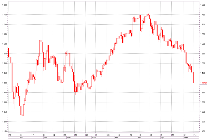
Fig. 1 - Interval chart in the form of Japanese candles RTS index. Period - day.
')
For reference: each figure on the chart shows us a certain period of time (in this case one day) and price movements over this period. We describe them:
- the opening price is the value of the price at the beginning of this period of time
- the closing price is the value of the price at the end of this period of time
- the maximum price is the maximum price for the entire period of time
- the minimum price is the minimum price for the entire period of time
- if the price went up (bullish trend) for this period - the body of the candle will be white (or transparent)
- if the price went down (bearish trend) for this period - the candle body will be black (or painted over) ^[6]

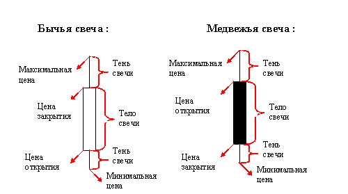
Fig. 2 - Japanese candles.

Really significant for predictions are changes in quotes. Therefore, after preprocessing, we will supply a number of percentage increments of quotes calculated by the formula X [t] / X [t-1] to the input of the neural network, where X [t] and X [t-1] are the closing prices of periods.

Fig. 3 - A series of percentage increments of quotes calculated by the formula X [t] / X [t-1].

But, since initially, the percentage increments have a Gaussian distribution, and of all the statistical distribution functions defined on a finite interval, the uniform entropy has the maximum entropy, then for this we recode the input variables so that all the examples in the training set carry approximately the same information load.

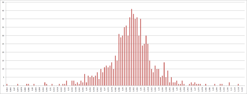
Fig. 4 - Distribution of percentage increments of quotes.

The algorithm here is the following: a segment from the minimum percentage increment to the maximum is divided into N segments, so that the range of values ​​of each segment includes an equal number of percentage increments of quotes.

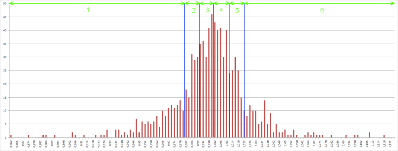
Fig. 5 - Borders of 6 segments, the number of percentage increments in each segment is equal.

Next, re-encode the percentage increments in the classes that identify each segment.

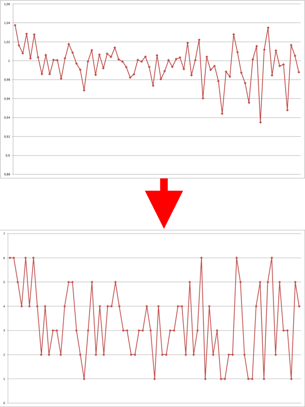
Fig. 6 - Recoding percentage increments.

And we get a uniform distribution.

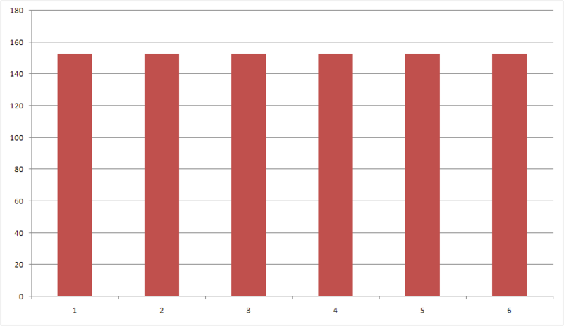
Fig. 7 - Uniform distribution.

The task of obtaining input images for the formation of a training set in problems of forecasting time series involves the use of the "window" method. This method involves the use of a “window” with a fixed size capable of moving through the time sequence of historical data, starting with the first element, and designed to access data of the time series, and the “window” of size N, having received such data, sends the elements to the input of the neural network 1 through N-1, and the N-th element is used as an output.

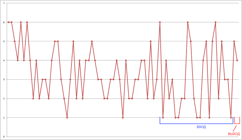
Fig. 8 - Window method.

The quality of the training sample is the higher, the less its inconsistency and the greater the repeatability. For the tasks of forecasting financial time series, the high inconsistency of the training sample is a sign that the description method was chosen poorly. Factors affecting inconsistency and repeatability:
1) the number of elements of the training sample - the more elements, the greater the inconsistency and repeatability;
2) the number of classes for which the percentage increments were recoded — with an increase, the inconsistency and repeatability decrease;
3) the depth of immersion in the financial time series ("window") - the greater the depth, the less inconsistency and less repeatability.
When creating a training sample, changing these parameters, it is necessary to find a balance in which the inconsistency level is minimal and the repeatability is maximum.

For a practical example, we will forecast the directions of increments of the RTS index from January 16, 2012, to April 17, 2012, the period is a day.

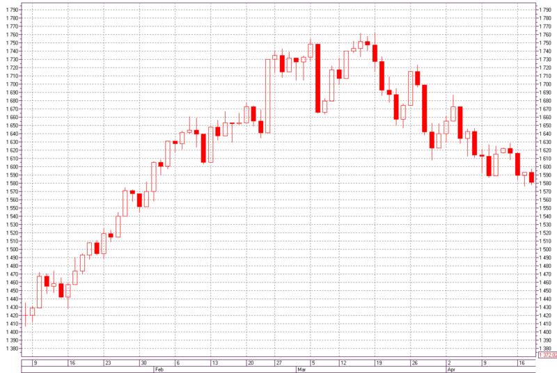
Fig. 9 - Schedule of the RTS index from January 8, 2012 to April 18, 2012, the period is a day.

Let's create a collection of neural networks that showed the best results (more than 70% of correctly predicted directions for changing the value of the index) on the test set (the last 50 periods). Every 5 periods, the collection is re-created, already predicted periods are included in the test set. The neural networks in the collection are not of the same type - each one has a training sample size, the number of classes for which the percentage increments are recoded, the immersion depth (“window”) and the number of neurons in the hidden layer so that the current market situation is most accurately predicted (the last 50 periods ).
The basic architecture of the used neural networks is a multilayer perceptron with one hidden layer. There is an excellent pre-built implementation in the ALGLIB library ^[7] . As a learning algorithm, we use the L-BFGS algorithm (limited memory BFGS), a quasi-Newtonian method with a time consuming iteration linear in the number of weight coefficients WCount and size of the training set, and moderate requirements for additional memory - O (WCount).

Sample collection:

Forecast from: 01/16/2012 to: 01/20/2012
Number of networks: 16
Network settings:
Input: 3 Concealed layer: 18 Number of classes: 4 Training sample length: 200 Result per vol. vyb .: 74,6 Result on test vyb .: 72,5
Input: 3 Concealed layer: 19 Number of classes: 4 Length of the training sample: 200 Result per vol. vyb .: 74,6 Result on test vyb .: 72,5
Input: 3 Concealed layer: 20 Number of classes: 4 Training sample length: 200 Result per vol. vyb .: 74,6 Result on test vyb .: 72,5
Input: 4 Concealed layer: 18 Number of classes: 4 Training sample length: 200 Result per vol. vyb .: 75,6 Result on test vyb .: 74,5
Input: 4 Concealed layer: 20 Number of classes: 4 Training sample length: 200 Result per vol. vyb .: 74,1 Result on test vyb .: 72,5
Input: 5 Concealed layer: 19 Number of classes: 4 Training sample length: 200 Result per vol. vyb .: 74,6 Result on test vyb .: 70,6
Entry: 5 Covered layer: 20 Number of classes: 4 Training sample length: 200 Result per vol. vyb .: 76,1 Result on test vyb .: 72,5
Input: 4 Concealed layer: 18 Number of classes: 5 Training sample length: 200 Result per vol. vyb .: 67,2 Result on test vyb .: 74,5
Input: 5 Build layer: 18 Number of classes: 5 Training sample length: 200 Result per vol. vyb .: 70,6 Result on test vyb .: 74,5
Entry: 5 Concealed layer: 19 Number of classes: 5 Training sample length: 200 Result per vol. vyb .: 76,6 Result on test vyb .: 74,5
Entry: 5 Reserved layer: 20 Number of classes: 5 Length of the training sample: 200 Result per vol. vyb .: 76,1 Result on test vyb .: 74,5
Input: 3 Concealed layer: 18 Number of classes: 4 Training sample length: 270 Result per vol. vyb .: 74,9 Result on test vyb .: 70,6
Input: 3 Concealed layer: 19 Number of classes: 4 Training sample length: 270 Result per vol. vyb .: 74,9 Result on test vyb .: 70,6
Input: 3 Concealed layer: 20 Number of classes: 4 Training sample length: 270 Result per vol. vyb .: 74,9 Result on test vyb .: 70,6
Input: 5 Build layer: 18 Number of classes: 4 Length of the training sample: 340 Result per vol. vyb .: 78,0 Result on test vyb .: 70,6
Input: 5 Concealed layer: 19 Number of classes: 4 Training sample length: 340 Result per vol. vyb .: 79,5 Result on test vyb .: 74,5


Parameters of all used collections can be found in the file

Since we forecast the direction of the RTS index change, we use the simplest strategy - we open a position at the closing price of the current period and close it at the closing price of the forecast period, fixing a profit or loss.

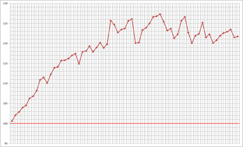
Fig. 10 - The result of the work.

The result of work from 16/01/2012 to 04/17/2012: 77% of correctly predicted directions of changes in the index value.