Noise reduction as a diffusion task
Hello, Habr.
Recently, it just so happened that I read a lecture in my old lyceum on the topic of why they study mathematics and what can then be done with it a little more applied. For schoolchildren of the 10th grade, it turned out to be a bit complicated, perhaps. I hope this topic will be interesting to someone from the community (here the option is a bit more complicated than what I read in the lyceum, but I do not think this is a problem).
So. It will be about image processing, in particular, about one of the simplest, but descriptively beautiful, method of suppressing noise in an image.
')
Not so long ago, I discovered for myself how much physics is in image processing. I was very interested in this, in view of the fact that these two branches of science in my head never crossed. In this article I will present how to remove noise from an image by solving the problem of mass transfer on a plane.
First, we specify what we will consider the image. For ease of description, we will now consider only b / w images.
We will represent them as a saturation matrix.

Thus, each pixel of the image corresponds to an element of the matrix. The values in the matrix are
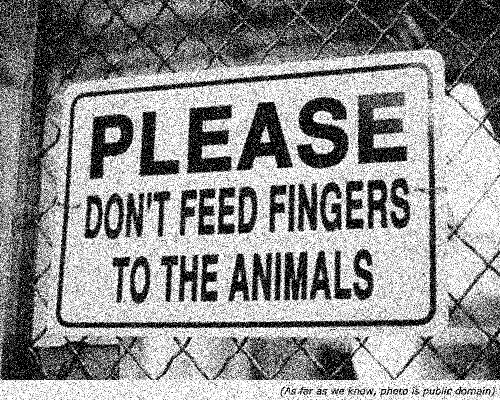
Take some image and add noise to it (this is easier than looking for an image already with noise, since you can check how well the algorithm copes with noise by setting different noise intensity). We get something like this:
To further explain the method, I need to enter some notation:
First, we will further consider our image as a function of pixel coordinates. So, if we want to say that a pixel with
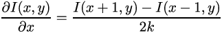
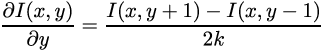
Further, if we have a function, then we can take a derivative from it and then it will be useful to us. Since we have a discrete function, that is, it is defined in the cells, with a fixed step between them, we can write it as (since the function is two-dimensional, then the derivatives, respectively, are two):
Here
Thus, the derivatives will also be matrices of the same size as the original image:


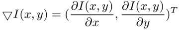
Having derivatives in both coordinates it is logical to calculate the gradient:
And its value:
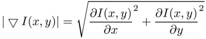
The magnitude of the gradient can be displayed as an image:
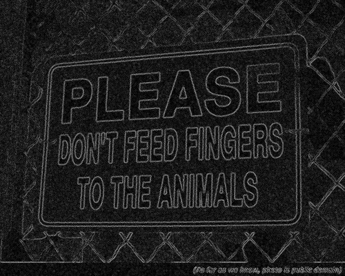
Now, carefully look at the magnitude of the gradient. It has great value where we store the information we need.
To rid the image of noise, it is logical to blur it. However, when blurring lost important details. That is, we would like to limit the blur in areas where the gradient is large enough. There was only a question how to do it.
This is where the wonderful physical process of diffusion comes to our aid. Imagine the image matrix as an indicator of the presence of mass in one or another point of the plane. The diffusion process consists in the fact that the mass “spreads” from the points with its large concentration to the points with small. In the process of diffusion there is the concept of flow, which obeys the so-called Fick's law:

Where
We also write the law of conservation of mass, which says that the difference between the incoming and outgoing flows is equal to the change in mass at the point:
If the flow is not limited, that is,
One of the simplest methods is to limit the magnitude of the flow, without limiting its direction. About him and we will continue.
Let us introduce into consideration some decreasing function, to the input of which we will supply the magnitude of the gradient. This function at this stage will be a diffusion tensor:

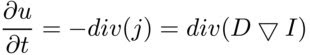
Then the mass conservation equation takes the form:

Next, we write out all the formulas (I’ll, perhaps, omit this step) and write the final equation with which you can find the solution to the problem:

Thus, we have obtained an iteration scheme that is stable for the parameter values of
In the end, we get an image that has retained almost all the important details and lost almost all the noise.
UPD: I sincerely apologize, the images were mixed up. Replaced the image that was previously that is obtained as a result of image processing with as much noise as presented in the article. Once again, I apologize.
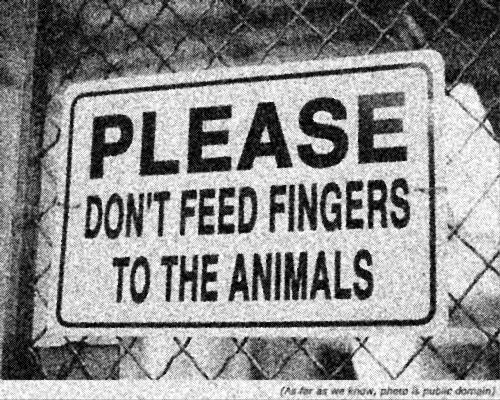
For comparison - the original and the version with noise (once again):

Literature:
PS If you find inaccuracies - I will be glad to hear criticism and suggestions.
Recently, it just so happened that I read a lecture in my old lyceum on the topic of why they study mathematics and what can then be done with it a little more applied. For schoolchildren of the 10th grade, it turned out to be a bit complicated, perhaps. I hope this topic will be interesting to someone from the community (here the option is a bit more complicated than what I read in the lyceum, but I do not think this is a problem).
So. It will be about image processing, in particular, about one of the simplest, but descriptively beautiful, method of suppressing noise in an image.
')
Not so long ago, I discovered for myself how much physics is in image processing. I was very interested in this, in view of the fact that these two branches of science in my head never crossed. In this article I will present how to remove noise from an image by solving the problem of mass transfer on a plane.
Image view
First, we specify what we will consider the image. For ease of description, we will now consider only b / w images.
We will represent them as a saturation matrix.
Thus, each pixel of the image corresponds to an element of the matrix. The values in the matrix are
float numbers from the interval [0,255] .Take some image and add noise to it (this is easier than looking for an image already with noise, since you can check how well the algorithm copes with noise by setting different noise intensity). We get something like this:
Image as a function
To further explain the method, I need to enter some notation:
First, we will further consider our image as a function of pixel coordinates. So, if we want to say that a pixel with
I(x,y)==255Further, if we have a function, then we can take a derivative from it and then it will be useful to us. Since we have a discrete function, that is, it is defined in the cells, with a fixed step between them, we can write it as (since the function is two-dimensional, then the derivatives, respectively, are two):
Here
k==1 because the difference between adjacent pixels = 1 pixel.Thus, the derivatives will also be matrices of the same size as the original image:
Having derivatives in both coordinates it is logical to calculate the gradient:
And its value:
The magnitude of the gradient can be displayed as an image:
Now, carefully look at the magnitude of the gradient. It has great value where we store the information we need.
To rid the image of noise, it is logical to blur it. However, when blurring lost important details. That is, we would like to limit the blur in areas where the gradient is large enough. There was only a question how to do it.
Connection to the diffusion process
This is where the wonderful physical process of diffusion comes to our aid. Imagine the image matrix as an indicator of the presence of mass in one or another point of the plane. The diffusion process consists in the fact that the mass “spreads” from the points with its large concentration to the points with small. In the process of diffusion there is the concept of flow, which obeys the so-called Fick's law:
Where
D is the diffusion tensor, which specifies the direction and magnitude of the diffusion.We also write the law of conservation of mass, which says that the difference between the incoming and outgoing flows is equal to the change in mass at the point:
If the flow is not limited, that is,
D==1 - the mass will spread in all directions evenly, that is, we will get the equivalent of Gaussian blur, which means we will lose important image details. We are interested in the method by which the flow can be limited.One of the simplest methods is to limit the magnitude of the flow, without limiting its direction. About him and we will continue.
Let us introduce into consideration some decreasing function, to the input of which we will supply the magnitude of the gradient. This function at this stage will be a diffusion tensor:
Then the mass conservation equation takes the form:
Next, we write out all the formulas (I’ll, perhaps, omit this step) and write the final equation with which you can find the solution to the problem:
Thus, we have obtained an iteration scheme that is stable for the parameter values of
tau<=0.25 . It is rather slow, since the method is basic and the more successful algorithms are based on it.Result
In the end, we get an image that has retained almost all the important details and lost almost all the noise.
UPD: I sincerely apologize, the images were mixed up. Replaced the image that was previously that is obtained as a result of image processing with as much noise as presented in the article. Once again, I apologize.
For comparison - the original and the version with noise (once again):
Literature:
- P. Perona, J. Malik: Scale-space and edge detection using anisotropic diffusion. IEEE
Transactions on Pattern Analysis and Machine Intelligence 12 (7): 629-639, 1990. - J. Weickert: Anisotropic Diffusion in Image Processing. Teubner, Stuttgart, 1998. The book is
not available anymore, but it is the PhD of Joachim Weickert,
book, is available on his website. - T. Brox: Lectures on Computer Vision. Freiburg im Breisgau, 2011
PS If you find inaccuracies - I will be glad to hear criticism and suggestions.
Source: https://habr.com/ru/post/144288/
All Articles