As I pulled the map back into the table
Again - because somehow more than 2 years ago I was already doing this exercise. It was a long and difficult process:
blogs.technet.com/b/isv_team/archive/2010/01/18/3306462.aspx
blogs.technet.com/b/isv_team/archive/2010/01/21/3307201.aspx
blogs.technet.com/b/isv_team/archive/2010/01/23/3307719.aspx
blogs.technet.com/b/isv_team/archive/2010/01/24/3307804.aspx
Since then, science has stepped far forward. In this post, we will again load the map of our vast Motherland into SQL Server, this time much easier and more elegant thanks to the authors of the maps, the new features of SQL Server and the independent developers, to whom all many thanks. We will need:
1. Suitable card
2. SQL Server 2012 (can Express)
3. A tool to convert maps from its original format to SQL Server.
Most of the work will be undertaken by the wonderful free utility Shape2SQL , which was written by the Danish MVP Morten Ødegaard Nielsen, God bless him, working GIS Lead Software Engineer in ESRI. The company ESRI (Environmental Systems Research Institute) is known for software products of the ArcGIS family, which are widely distributed, including in Russia. The vector format of shape files was introduced for ArcView GIS version 2 in the early 90s, and today due to its prevalence it has become the de facto standard for exchanging data between geographic information systems. As the name implies, Tula can load shapefiles in SQL Server 2008 and higher. In this post 2012 is used because of the support of geometric / geographical aggregates that appeared in it - it will come in handy later. In 2008, I would have to write a cursor.
Note 1. In addition to the .shp import utility in SQL Server, SqlSpatialTools v1.3.0 (348 kb) (build 3759) on SharpGIS includes the SqlSpatial Query Tool map visualization client on WPF and Silverlight, which is much richer in its capabilities than the geographic panel SSMS results.
Note 2. Both tools, as the author warns, are not intended for commercial use, since written by him for his own needs or pleasure.
Note 3. An open source .NET library that can parse shape files is located here .
It remains to find a shape-file with the administrative-territorial division of the Russian Federation. Maps of Russian regions in various formats, including .shp, were found on the GIS-Lab laboratory website : this layer is licensed under the CC-BY license , allowing any use, including transfer, modification, use in commercial projects, subject to the mention of authorship and availability hyperlinks. The data sources for the maps were the Federal Service for State Registration, Cadastre and Cartography ( Rosreestr ) - the boundaries of the subjects, OpenStreerMap Russia ( OSM ) - the Land Border of Russia, except for the Kaliningrad Region + the boundary of Moscow, VMap0 - the coastline + the borders of the Kaliningrad Region and the initiative group project GIS-Lab.info , for which they, too, expressed deep appreciation.
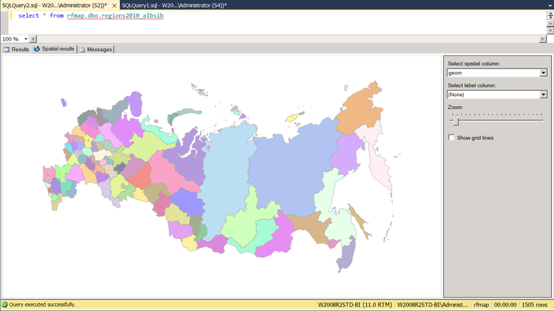
GIS-Lab maps are shown in 3 projections : WGS 1984 (GPS), Pulkovo-1942 and Albers-Siberia. To display the territory of Russia, the third is best suited:
')
Pic.1
than the first two:
Pic2
Unfortunately, I did not manage to find in the sys.spatial_reference_systems an equal Albers conic projection with a central meridian = 1050 E based on the Krasovsky spheroid, so it can be dragged into SQL Server as geometry and used, for example, as a means of report visualization. The first two are imported into the geography type (SRID = 4326, 4284), and can be used for cartographic calculations.
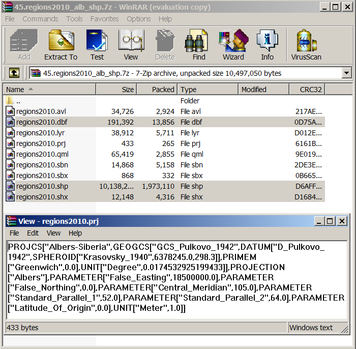
To import the map, we need three files:
Pic.3
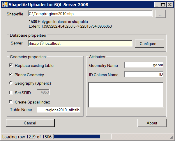
The .shp / .shx files are fed to the input of the awesome Tule Shape2SQL, which was mentioned above. Specify the full name of the shapefile, the connection to SQL Server, the name of the table into which the data from the shapefile will be imported, the name of the geospatial column in the table, the name of the column that will act as the primary key. If the table did not exist, it is created. Importing data in the Albers Siberia projection as a geography is not possible, because SQL Server does not know such a SRIDa and incorrectly converts the coordinates — it is by the SqlGeography type — so we import them as geometry. If you wish, you can immediately build a geospatial index. Click the Upload to Database button, and the dbo.regions2010_albsib table is successfully created and populated with data:
Pic.4
You can make
and use the import / export wizard. In principle, it automatically associates the source and destination fields with the same name, but once again you can make sure of this by clicking
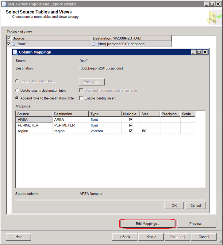
Pic.5
If the length of the region is unknown in advance, i.e. there is no dbf reader at hand, and parsing with a binary editor is a lazy header, you can lay the maximum length, and after import cut it. The dbf import is successful, and along with the table of cartographic objects in the SQL Server database, a table of signatures to them appears:

Pic.6
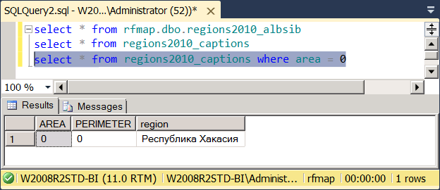
The entries in the table of map objects regions2010_albsib are connected with the table of signatures regions2010_captions exclusively by the physical order, which is not good, because nobody promised that the import / export wizard transfers the records in the same order as they were in dbf. The best way out of this situation would be the presence of the RC in dbf and in shp, which would make it easy to compare them and, by the way, would save the author of Shape2SQL from the need to invent a surrogate ID. But such cards are dealt. Attention is drawn to the fact that the records of signatures are 1506, and the records of cartographic objects are 1505 (Fig. 1), although during the loading process in Fig. 4, Shape2SQL also wrote that there were 1506. Where did another one go? Here it turns out one serious failure zatotnoy Tula, which is that it does not load empty objects. She skips them, and the records in the table of cartographic objects may turn out to be smaller than the signatures, as a result of which the correspondence in physical order moves to the devil's grandmother, because how to understand which records by the number were dropped from the middle? It is good that the area and perimeter columns are present, from which you can calculate the record corresponding to the empty map object in the captions:
Pic.7
After its removal from the table of signatures, a hole appears from the table of deletions
I strongly hope that the regions2010_albsib table Nielsen also receives in the order of physical scanning of objects. Then its ID field can be associated with the regions2010_captions table (n field). The number of cartographic objects exceeds the actual number of regions, because, as we see from the signatures, one region may consist of more than one landfill: Moscow and Zelenograd, coastal territory and islands, etc. For example,

Fig.8
So, they need to be combined, aggregated on the basis of the same region:
This code illustrates two new features in SQL Server 2012: sequences and geospatial aggregates.
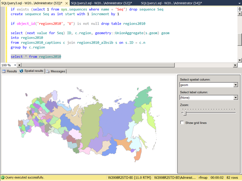
Fig.9
Judging by the color seems to be true. So, with the binding of signatures and polygons, we were not mistaken.
Despite the fact that polygons belonging to the same region are painted with the same color, these are separate objects, of which a region of the same type (multipolygon) constitutes the same type of geometric collection. You can verify this by running the query

Pic.10
To deploy them from collection to table for the selected region, I wrote a simple function:
which allows from the aggregate, in fact, table regions2010 again to return to the original regions2010_albsib:

Figure 11
Actually, this is not exactly her. Please note that the detailed polygons are already 1503, and not 1505. I explain this by the fact that there were two pairs of intersecting polygons or three intersecting polygons within the same region, which merged into one. Let's check:
Indeed, there are seven such intersections in total, of which 5 point ones, which, when combined, do not collapse into one polygon, and two pairs of adjacent polygons, i.e. having a common border in the form of a broken line. Each of these pairs merged into one polygon, so their number was reduced by 2:

Fig.12
In conclusion, we consider the practical action of the Reduce () method. Please note that drawing a region2010 map (Figure 9) takes a delay of 2-3 seconds. This is caused by a significant number of points - about thousands or even tens of thousands - defining the contour of each region. For a map of the size that will be shown in the report, such thoroughness is superfluous, unnecessarily increasing the rendering time. For roughening, the Reduce () method is used, which operates according to the Douglas-Pecker algorithm. The greater the value of the parameter, the stronger the coarsening (we have analyzed the tolerant methods here ). For example,

Fig.13
Thus,

Fig.14
blogs.technet.com/b/isv_team/archive/2010/01/18/3306462.aspx
blogs.technet.com/b/isv_team/archive/2010/01/21/3307201.aspx
blogs.technet.com/b/isv_team/archive/2010/01/23/3307719.aspx
blogs.technet.com/b/isv_team/archive/2010/01/24/3307804.aspx
Since then, science has stepped far forward. In this post, we will again load the map of our vast Motherland into SQL Server, this time much easier and more elegant thanks to the authors of the maps, the new features of SQL Server and the independent developers, to whom all many thanks. We will need:
1. Suitable card
2. SQL Server 2012 (can Express)
3. A tool to convert maps from its original format to SQL Server.
Most of the work will be undertaken by the wonderful free utility Shape2SQL , which was written by the Danish MVP Morten Ødegaard Nielsen, God bless him, working GIS Lead Software Engineer in ESRI. The company ESRI (Environmental Systems Research Institute) is known for software products of the ArcGIS family, which are widely distributed, including in Russia. The vector format of shape files was introduced for ArcView GIS version 2 in the early 90s, and today due to its prevalence it has become the de facto standard for exchanging data between geographic information systems. As the name implies, Tula can load shapefiles in SQL Server 2008 and higher. In this post 2012 is used because of the support of geometric / geographical aggregates that appeared in it - it will come in handy later. In 2008, I would have to write a cursor.
Note 1. In addition to the .shp import utility in SQL Server, SqlSpatialTools v1.3.0 (348 kb) (build 3759) on SharpGIS includes the SqlSpatial Query Tool map visualization client on WPF and Silverlight, which is much richer in its capabilities than the geographic panel SSMS results.
Note 2. Both tools, as the author warns, are not intended for commercial use, since written by him for his own needs or pleasure.
Note 3. An open source .NET library that can parse shape files is located here .
It remains to find a shape-file with the administrative-territorial division of the Russian Federation. Maps of Russian regions in various formats, including .shp, were found on the GIS-Lab laboratory website : this layer is licensed under the CC-BY license , allowing any use, including transfer, modification, use in commercial projects, subject to the mention of authorship and availability hyperlinks. The data sources for the maps were the Federal Service for State Registration, Cadastre and Cartography ( Rosreestr ) - the boundaries of the subjects, OpenStreerMap Russia ( OSM ) - the Land Border of Russia, except for the Kaliningrad Region + the boundary of Moscow, VMap0 - the coastline + the borders of the Kaliningrad Region and the initiative group project GIS-Lab.info , for which they, too, expressed deep appreciation.
GIS-Lab maps are shown in 3 projections : WGS 1984 (GPS), Pulkovo-1942 and Albers-Siberia. To display the territory of Russia, the third is best suited:
')
Pic.1
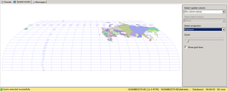
than the first two:
Pic2
Unfortunately, I did not manage to find in the sys.spatial_reference_systems an equal Albers conic projection with a central meridian = 1050 E based on the Krasovsky spheroid, so it can be dragged into SQL Server as geometry and used, for example, as a means of report visualization. The first two are imported into the geography type (SRID = 4326, 4284), and can be used for cartographic calculations.
To import the map, we need three files:
Pic.3
The .shp / .shx files are fed to the input of the awesome Tule Shape2SQL, which was mentioned above. Specify the full name of the shapefile, the connection to SQL Server, the name of the table into which the data from the shapefile will be imported, the name of the geospatial column in the table, the name of the column that will act as the primary key. If the table did not exist, it is created. Importing data in the Albers Siberia projection as a geography is not possible, because SQL Server does not know such a SRIDa and incorrectly converts the coordinates — it is by the SqlGeography type — so we import them as geometry. If you wish, you can immediately build a geospatial index. Click the Upload to Database button, and the dbo.regions2010_albsib table is successfully created and populated with data:
Pic.4
You can make
select * from rfmap.dbo.regions2010_albsib and make sure that everything is OK on the Spatial results tab in SSMS (see Figure 1). However, the number of entries in the table is slightly higher than the number of regions of Russia. To understand what's the matter, we need a third file - dbf, containing metadata to the map. How to load dbf in SQL Server, we went through in the previous post . Create a tableCREATE TABLE dbo.regions2010_captions (
ID int IDENTITY(1,1) NOT NULL,
AREA float NULL,
PERIMETER float NULL,
region varchar(50) NULL
)and use the import / export wizard. In principle, it automatically associates the source and destination fields with the same name, but once again you can make sure of this by clicking
Pic.5
If the length of the region is unknown in advance, i.e. there is no dbf reader at hand, and parsing with a binary editor is a lazy header, you can lay the maximum length, and after import cut it. The dbf import is successful, and along with the table of cartographic objects in the SQL Server database, a table of signatures to them appears:
Pic.6
The entries in the table of map objects regions2010_albsib are connected with the table of signatures regions2010_captions exclusively by the physical order, which is not good, because nobody promised that the import / export wizard transfers the records in the same order as they were in dbf. The best way out of this situation would be the presence of the RC in dbf and in shp, which would make it easy to compare them and, by the way, would save the author of Shape2SQL from the need to invent a surrogate ID. But such cards are dealt. Attention is drawn to the fact that the records of signatures are 1506, and the records of cartographic objects are 1505 (Fig. 1), although during the loading process in Fig. 4, Shape2SQL also wrote that there were 1506. Where did another one go? Here it turns out one serious failure zatotnoy Tula, which is that it does not load empty objects. She skips them, and the records in the table of cartographic objects may turn out to be smaller than the signatures, as a result of which the correspondence in physical order moves to the devil's grandmother, because how to understand which records by the number were dropped from the middle? It is good that the area and perimeter columns are present, from which you can calculate the record corresponding to the empty map object in the captions:
Pic.7
After its removal from the table of signatures, a hole appears from the table of deletions
delete from regions2010_captions where area = 0 . It’s good that in our case it was the penultimate record, and the number of the latter can simply be changed to 1505. Nevertheless, we honestly enumerate the signatures in a new way in increasing order of ID, as if there were several deleted records and they would be scattered somewhere in the middle.alter table regions2010_captions add n int
;with cte as (select *, row_number() over (order by ID) n1 from regions2010_captions) update cte set n = n1
alter table regions2010_captions drop column IDI strongly hope that the regions2010_albsib table Nielsen also receives in the order of physical scanning of objects. Then its ID field can be associated with the regions2010_captions table (n field). The number of cartographic objects exceeds the actual number of regions, because, as we see from the signatures, one region may consist of more than one landfill: Moscow and Zelenograd, coastal territory and islands, etc. For example,
select s.geom from regions2010_captions c join regions2010_albsib s on s.ID = cn where c.region = ' ' :Fig.8
So, they need to be combined, aggregated on the basis of the same region:
if exists (select 1 from sys.sequences where name = 'Seq') drop sequence Seq
create sequence Seq as int start with 1 increment by 1

if object_id('regions2010', 'U') is not null drop table regions2010

select (next value for Seq) ID, c.region, geometry::UnionAggregate(s.geom) geom
into regions2010
from regions2010_captions c join regions2010_albsib s on s.ID = cn
group by c.region

select * from regions2010
This code illustrates two new features in SQL Server 2012: sequences and geospatial aggregates.
Fig.9
Judging by the color seems to be true. So, with the binding of signatures and polygons, we were not mistaken.
Despite the fact that polygons belonging to the same region are painted with the same color, these are separate objects, of which a region of the same type (multipolygon) constitutes the same type of geometric collection. You can verify this by running the query
select ID, Region, geom.STGeometryType(), geom.STNumGeometries() from regions2010 :Pic.10
To deploy them from collection to table for the selected region, I wrote a simple function:
if object_id('dbo.ufnGeometries', 'TF') is not null drop function dbo.ufnGeometries
go
create function dbo.ufnGeometries(@g geometry) returns @t table (id int identity(1, 1), g geometry) as begin
declare @i int = 1
while @i <= @g.STNumGeometries() begin
insert @t (g) values (@g.STGeometryN(@i))
set @i += 1
end
return
end
which allows from the aggregate, in fact, table regions2010 again to return to the original regions2010_albsib:
select r.ID, r.Region, f.ID, fg from regions2010 r cross apply dbo.ufnGeometries(geom) fFigure 11
Actually, this is not exactly her. Please note that the detailed polygons are already 1503, and not 1505. I explain this by the fact that there were two pairs of intersecting polygons or three intersecting polygons within the same region, which merged into one. Let's check:
with cte as (select s.ID, s.geom, c.region from regions2010_albsib s join regions2010_captions c on s.ID = cn)
select cte1.ID, cte1.geom, cte2.ID, cte2.geom, cte1.geom.STIntersection(cte2.geom).STGeometryType() from cte cte1 join cte cte2 on cte1.ID < cte2.ID and cte1.region = cte2.region
where cte1.geom.STIntersects(cte2.geom) = 1
Indeed, there are seven such intersections in total, of which 5 point ones, which, when combined, do not collapse into one polygon, and two pairs of adjacent polygons, i.e. having a common border in the form of a broken line. Each of these pairs merged into one polygon, so their number was reduced by 2:
Fig.12
In conclusion, we consider the practical action of the Reduce () method. Please note that drawing a region2010 map (Figure 9) takes a delay of 2-3 seconds. This is caused by a significant number of points - about thousands or even tens of thousands - defining the contour of each region. For a map of the size that will be shown in the report, such thoroughness is superfluous, unnecessarily increasing the rendering time. For roughening, the Reduce () method is used, which operates according to the Douglas-Pecker algorithm. The greater the value of the parameter, the stronger the coarsening (we have analyzed the tolerant methods here ). For example,
select ID, Region, geom.STNumPoints() [Points Total], geom.Reduce(100).STNumPoints() Reduce100, geom.Reduce(500).STNumPoints() Reduce500, geom.Reduce(1000).STNumPoints() Reduce1000 from regions2010Fig.13
Thus,
select ID, Region, geom.Reduce(1000) from regions2010 drawn in a select ID, Region, geom.Reduce(1000) from regions2010 any other, while maintaining the quality map visible for a given scale:Fig.14
Source: https://habr.com/ru/post/144006/
All Articles