Recommender systems: overfitting and regularization
Constantly declining popularity of previous publications encourages actions to help support popularity. I noticed that the popularity of the first publications considerably exceeds the subsequent ones; so try to reboot.
Throughout the previous series, we carefully considered the SVD method and even brought it to the program code; starting with this text, I will consider more general things. Of course, these things will always be closely connected with recommender systems, and I will talk about how they emerge in recommender systems, but I will try to focus on more general concepts of machine learning. Today - about overfitting and regularization.

I will start with the classic, but no less illustrative example. Let's open R (if anyone does not know, R is one of the best tools in the world for all sorts of statistics, machine learning and data processing in general; I highly recommend it) and generate some small simple dataset for ourselves. I'll take a simple cubic polynomial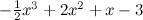 and add normally distributed noise to its points.
')
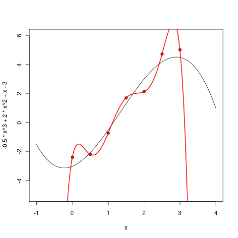
These points can now be drawn along with the ideal curve.
It turns out as shown:

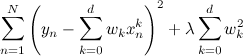
And now let's try to train a polynomial from this data. We will minimize the sum of squares of deviations of points from the polynomial (we will do the most usual classical regression), that is, we will look for such a polynomial p (x) that minimizes .
.
Of course, in R this is done by one team. First, we teach and draw a linear polynomial:
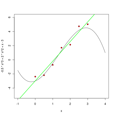
Then a second degree polynomial:
The third degree polynomial, as expected, is already quite similar to itself:

But what happens if you increase the degree further? In practice, we most likely will not know the “true degree of a polynomial”, i.e. true complexity of the model. It may seem that, by complicating the model, we will better approximate the existing points, and the results will be better and better, just to train the model will be harder and harder. Let's see if this is true.
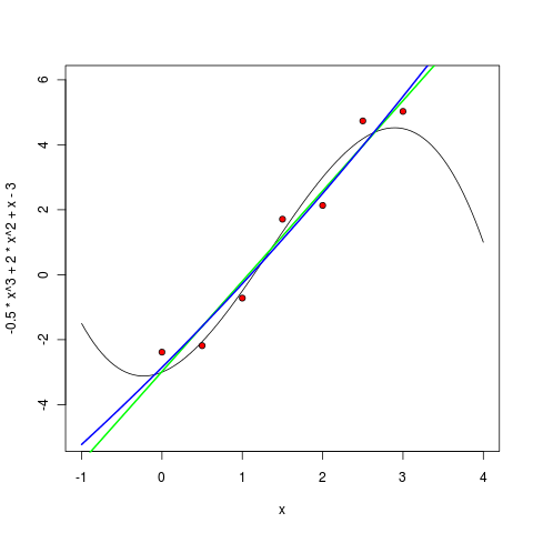
The fifth degree polynomial already looks very suspicious - it is, of course, still well-behaved between points, but it is already clear that it will not be good to extrapolate using this model - it starts to go too sharply to infinity as soon as the points end.
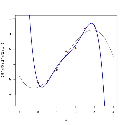
Starting from the sixth degree, we see the undoubted epic fail of our approach. The error that we wanted to minimize is now strictly equal to zero — after all, a polynomial of the sixth degree can be drawn through seven points! But the benefits of the resulting model, too, are probably strictly zero - now the polynomial not only badly extrapolates beyond the existing points, but even interpolates between them extremely strange, running far to local extremes where it is difficult to expect this from the points.
What happened? What happened in machine learning is called overfitting: we took a model in which there were too many parameters, and the model learned too well from the data, and most importantly, the predictive power — on the contrary, it suffered.
What to do? In the next series I will tell you how this can turn out to be more conceptual, but now let's just take it for granted: overfitting in this case is manifested in the fact that the resulting polynomials have too large coefficients. For example, here is a third degree polynomial that we taught:
 ,
,
but feel the difference - the sixth degree:
 .
.
Accordingly, it is possible to deal with this in a rather natural way: you just need to add a penalty to the objective function that would punish the model for too large coefficients:
 .
.
This overfitting would often occur in SVD if we allowed it to happen. Indeed, we introduce for each user and each product a number of free parameters equal to the number of factors (i.e. at least a few, and maybe a few dozen). Therefore, SVD without regularization is completely inapplicable - it will certainly be good to learn, but it will most likely be practically useless for predictions.
Regularizers in SVD work in the same way as in regular regression - we add a penalty, which is greater, the greater the size of the coefficients; in one of the previous series, I immediately followed the regularizers and wrote out the objective function:

The formulas of the gradient lift are given in the same place - the coefficient λ corresponds to the regularization in them.
However, while it all looks pretty mysterious - why would suddenly large coefficients be worse than small ones? In the future, I will talk about how you can look at this issue from a more conceptual Bayesian side.
Throughout the previous series, we carefully considered the SVD method and even brought it to the program code; starting with this text, I will consider more general things. Of course, these things will always be closely connected with recommender systems, and I will talk about how they emerge in recommender systems, but I will try to focus on more general concepts of machine learning. Today - about overfitting and regularization.
I will start with the classic, but no less illustrative example. Let's open R (if anyone does not know, R is one of the best tools in the world for all sorts of statistics, machine learning and data processing in general; I highly recommend it) and generate some small simple dataset for ourselves. I'll take a simple cubic polynomial
and add normally distributed noise to its points.> x <- c(0:6) / 2 > y_true <- -.5*x^3 + 2*x^2 + x – 3 > err <- rnorm( 7, mean=0, sd=0.4 ) > y <- y_true + err > y [1] -2.3824664 -2.1832300 -0.7187618 1.7105423 2.1338531 4.7356023 5.0291615 ')
These points can now be drawn along with the ideal curve.
> curve(-.5*x^3 + 2*x^2 + x - 3, -1, 4, ylim=c(-5,6) ) > points(x, y, pch=21, bg="red") It turns out as shown:
And now let's try to train a polynomial from this data. We will minimize the sum of squares of deviations of points from the polynomial (we will do the most usual classical regression), that is, we will look for such a polynomial p (x) that minimizes
.Of course, in R this is done by one team. First, we teach and draw a linear polynomial:
> m1 <- lm ( y ~ poly(x, 1, raw=TRUE) ) > pol1 <- function(x) m1$coefficients[1] + m1$coefficients[2] * x > curve(pol1, col="green", lwd=2, add=TRUE) Then a second degree polynomial:
> m2 <- lm ( y ~ poly(x, 2, raw=TRUE) ) > pol2 <- function(x) m2$coefficients[1] + m1$coefficients[2] * x + m1$coefficients[3] * (x^2) > curve(pol2, col="blue", lwd=2, add=TRUE) The third degree polynomial, as expected, is already quite similar to itself:
But what happens if you increase the degree further? In practice, we most likely will not know the “true degree of a polynomial”, i.e. true complexity of the model. It may seem that, by complicating the model, we will better approximate the existing points, and the results will be better and better, just to train the model will be harder and harder. Let's see if this is true.
The fifth degree polynomial already looks very suspicious - it is, of course, still well-behaved between points, but it is already clear that it will not be good to extrapolate using this model - it starts to go too sharply to infinity as soon as the points end.
Starting from the sixth degree, we see the undoubted epic fail of our approach. The error that we wanted to minimize is now strictly equal to zero — after all, a polynomial of the sixth degree can be drawn through seven points! But the benefits of the resulting model, too, are probably strictly zero - now the polynomial not only badly extrapolates beyond the existing points, but even interpolates between them extremely strange, running far to local extremes where it is difficult to expect this from the points.
What happened? What happened in machine learning is called overfitting: we took a model in which there were too many parameters, and the model learned too well from the data, and most importantly, the predictive power — on the contrary, it suffered.
What to do? In the next series I will tell you how this can turn out to be more conceptual, but now let's just take it for granted: overfitting in this case is manifested in the fact that the resulting polynomials have too large coefficients. For example, here is a third degree polynomial that we taught:
,but feel the difference - the sixth degree:
.Accordingly, it is possible to deal with this in a rather natural way: you just need to add a penalty to the objective function that would punish the model for too large coefficients:
.This overfitting would often occur in SVD if we allowed it to happen. Indeed, we introduce for each user and each product a number of free parameters equal to the number of factors (i.e. at least a few, and maybe a few dozen). Therefore, SVD without regularization is completely inapplicable - it will certainly be good to learn, but it will most likely be practically useless for predictions.
Regularizers in SVD work in the same way as in regular regression - we add a penalty, which is greater, the greater the size of the coefficients; in one of the previous series, I immediately followed the regularizers and wrote out the objective function:
The formulas of the gradient lift are given in the same place - the coefficient λ corresponds to the regularization in them.
However, while it all looks pretty mysterious - why would suddenly large coefficients be worse than small ones? In the future, I will talk about how you can look at this issue from a more conceptual Bayesian side.
Source: https://habr.com/ru/post/143455/
All Articles